Demand, Supply, and Market Equilibrium: Explained

The Marketplace: A Framework for Interaction

Before we can analyze demand and supply, we need to understand the environment where they interact: the market. In economics, a market isn't necessarily a physical place; it's any situation that brings together buyers and sellers of a particular good or service.

The model we will build today works best under a specific set of idealized conditions known as perfect competition. The key assumptions are:

• There are many buyers and many sellers.
• The product is generic or standardized (one seller's product is identical to another's).
• No single buyer or seller can influence the market price. They are all price takers.

While few real-world markets are truly "perfect," this model provides a powerful and clear baseline for understanding market forces.

Demand: The Buyer's Side of the Market

Demand refers to the quantity of a good that consumers are both willing and able to purchase at different prices during a specific period. The core principle governing demand is the Law of Demand.

The Law of Demand states that, other things being equal, there is an inverse relationship between the price of a good and the quantity demanded. Simply put:

• When the price of a good falls, the quantity demanded increases.
• When the price of a good rises, the quantity demanded decreases.

This relationship gives the demand curve its characteristic downward slope when plotted on a graph with price on the vertical axis and quantity on the horizontal axis.

Supply: The Seller's Side of the Market

Supply is the counterpart to demand. It refers to the quantity of a good that producers are both willing and able to offer for sale at different prices during a specific period. The governing principle here is the Law of Supply.

The Law of Supply states that, other things being equal, there is a direct relationship between the price of a good and the quantity supplied. The logic is driven by profit:

• When the price of a good rises, producers are willing to supply more because it's more profitable.
• When the price of a good falls, producers supply less.

This positive relationship gives the supply curve its upward slope.

Market Equilibrium: Where Supply Meets Demand

Now, let's bring both sides of the market together. The point where the supply curve and the demand curve intersect is called market equilibrium. The price at this intersection is the equilibrium price, and the quantity is the equilibrium quantity.

At this point, the market is "cleared": the quantity that buyers want to purchase is exactly equal to the quantity that sellers want to sell. There is no pressure for the price to change.

What happens if the price is not at equilibrium?

• Excess Supply (Surplus): If the market price is above the equilibrium price, sellers are willing to supply more than buyers are willing to purchase. This creates a surplus. To sell their excess inventory, sellers will lower their prices, pushing the price down toward equilibrium.
• Excess Demand (Shortage): If the market price is below the equilibrium price, buyers want to purchase more than sellers are willing to supply. This creates a shortage. With many buyers competing for few goods, sellers can raise their prices, pushing the price up toward equilibrium.

This automatic adjustment process is what Adam Smith famously called the "invisible hand" of the market.

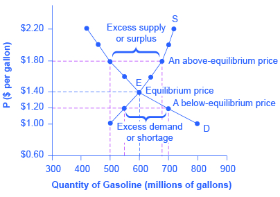
This graph illustrates market equilibrium in the gasoline market. At the equilibrium price of $1.40, quantity supplied equals quantity demanded. Any price above this (e.g., $1.80) creates a surplus, while any price below it (e.g., $1.20) creates a shortage. The market naturally adjusts back towards equilibrium.

To see this adjustment mechanism explained in detail, the following video offers an excellent breakdown of how markets self-correct from states of disequilibrium.

Shifts vs. Movements: A Crucial Distinction

So far, we have discussed how changes in a good's own price cause movements along the existing demand and supply curves. But what happens when an external factor changes? This causes the entire curve to shift. This is perhaps the most critical concept in applying this model.

A change in demand (or supply) is a shift of the entire curve, meaning that at any given price, a different quantity is demanded (or supplied). A change in quantity demanded (or supplied) is a movement along a fixed curve caused only by a change in the good's own price.

To analyze the impact of any event on a market, you can use a simple, algorithmic "three-step process":

1. Decide whether the event shifts the supply curve, the demand curve, or both.
2. Decide in which direction the curve shifts (right for an increase, left for a decrease).
3. Use the supply-and-demand diagram to see how the shift changes the equilibrium price and quantity.

For a quick and dynamic recap of all these concepts—the laws of demand and supply, the shifters, and equilibrium changes—the following video is an excellent summary.

Application: The Indian Onion Crisis

Let's apply this framework to a real-world Indian example, which is a key part of your learning goal.

This infographic shows the sharp spike in onion prices in India during 2013. We can use our demand-and-supply model to understand why this happened.

The infographic attributes the problem to "unusual late monsoon rains" and "hoarding by Traders." Let's analyze these using our three-step process.

1. Which curve shifts?

   • Unusual late monsoon rains: This is an adverse weather event that damages crops. It affects the ability of farmers to produce and bring onions to the market. This is a factor affecting supply.
   • Hoarding by Traders: This means sellers are deliberately holding back stock from the market, hoping to sell it later at a higher price. This also directly reduces the quantity available for sale at any given price, affecting supply.

2. In which direction does the curve shift?

   • Both factors—poor harvest and hoarding—reduce the amount of onions available on the market. This causes the supply curve to shift to the left.

3. What is the effect on equilibrium?

   • When the supply curve shifts to the left, while the demand curve remains relatively unchanged, the new intersection point (the new equilibrium) occurs at a higher price and a lower quantity. This is exactly what the graph shows: the price of onions soared from around Rs. 20-35 to Rs. 65 per kg.

This simple model elegantly explains the price spike that affected millions of households across the country.

Conclusion

In this lesson, we have built the foundational model of supply and demand, the primary tool for microeconomic analysis. You have learned how the interaction of buyers and sellers determines prices and how external events can cause those prices to change.

Here are the key takeaways:

• The Law of Demand describes an inverse relationship between price and quantity demanded (downward-sloping curve).
• The Law of Supply describes a direct relationship between price and quantity supplied (upward-sloping curve).
• Market Equilibrium occurs where supply equals demand. At this point, the market "clears," with a stable equilibrium price and quantity.
• Prices above equilibrium create a surplus, pushing prices down. Prices below equilibrium create a shortage, pushing prices up.
• It's crucial to distinguish between a movement along a curve (caused by a change in the good's own price) and a shift of the curve (caused by an external factor, or "determinant").

In our next lesson, we will move from the micro-foundations of a single market to the macro-level view of the entire economy. We will start with the single most important measure of economic activity: Gross Domestic Product (GDP), and learn to distinguish between its nominal and real values.