Summarizing Data with Pivot Tables

1. What is a Pivot Table?

At its core, a pivot table is an interactive tool that allows you to automatically summarize large amounts of data. Imagine you have a spreadsheet with thousands of rows of sales data, detailing every single transaction: date, product, region, salesperson, and sale amount. A business manager might ask, "What were our total sales per region last quarter?" or "Who were our top three salespeople in the banana category?"

Answering these questions by manually sorting, filtering, and using formulas like SUMIFS would be incredibly time-consuming and prone to error. A pivot table automates this process. It takes your flat, tabular data and allows you to "pivot" it—that is, to reorganize the rows and columns to view the data from different perspectives. You can group sales by region, then by salesperson, and see the total revenue for each, all with a few clicks.

For a quick conceptual overview of what pivot tables are and why they are so indispensable for an analyst, please read the introductory section of the following guide.

2. Building Your First Pivot Table: The Mechanics

Creating a pivot table is a straightforward process, but it relies on a well-structured data source and an understanding of its main components. Let's walk through the fundamental steps.

Data Preparation

First, your data must be in a "tabular" format. This means:

• Each column has a unique header.
• There are no completely blank rows or columns within your data.
• Each column contains a consistent data type (e.g., numbers in the 'Sales' column, dates in the 'Date' column).

A highly recommended best practice is to convert your data range into an Excel Table (you can do this by selecting a cell in your data and pressing Ctrl+T). When you base a pivot table on an Excel Table, it automatically expands to include any new rows or columns you add to your source data, making it much easier to keep your analysis up to date.

The PivotTable Fields Pane

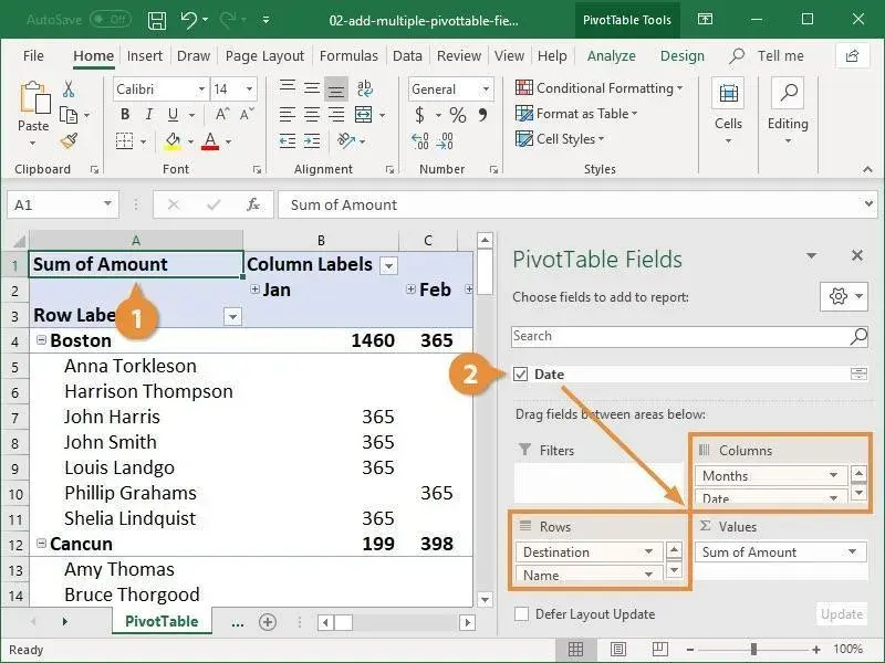
Once you insert a pivot table, you'll see the PivotTable Fields pane. This is your control center. It contains a list of all your data columns (fields) and four areas at the bottom:

1. Filters: Use this to apply a high-level filter to your entire report (e.g., filter the whole summary for a specific year or country).
2. Columns: Fields placed here become the column headers of your pivot table.
3. Rows: Fields placed here become the row labels. You can nest multiple fields to create hierarchies (e.g., Country, then State within each Country).
4. Values (∑): This is where you place the field you want to calculate (e.g., 'Sales Amount'). It will be summarized using a function like Sum, Count, or Average.

The following video from Kevin Stratvert provides an excellent step-by-step walkthrough of creating a basic pivot table. It covers converting data to a table, inserting the pivot table, and using the core areas of the Fields pane.

The image below shows a finished pivot table summarizing sales by Destination, Name, and Month. Notice how the fields in the pane on the right correspond to the structure of the table on the left.

3. Summarizing and Structuring Data for Analysis

Once you have the basic structure, the real power of pivot tables comes from how you can manipulate them to answer different questions.

Changing the Summary Calculation

By default, Excel will sum numerical values and count non-numerical (text) values. But you often need other calculations. For example, you might want to find the average sale amount, the largest single order (MAX), or the number of transactions (COUNT).

Creating Two-Dimensional Summaries

You can create more complex summaries by using both the Rows and Columns areas. For instance, you could place 'Region' in the Rows area and 'Product Category' in the Columns area to see a cross-tabulation of sales for each region by each category.

Showing Values in Different Ways

Beyond changing the summary function, you can also change how the values are displayed. This is extremely useful for analysis. For example, instead of showing the raw sum of sales for each salesperson, you can show their contribution as a percentage of the grand total. This instantly tells you what proportion of total revenue each person is responsible for.

The next segment of Kevin Stratvert's video demonstrates these essential techniques.

4. Refining Your Analysis: Sorting, Filtering, and Calculated Fields

To extract meaningful insights, you need to focus your analysis. Sorting and filtering are fundamental, but calculated fields take your analysis to the next level.

Sorting and Filtering

• Sorting: You can sort your pivot table to quickly identify key performers or areas. For example, sorting sales by 'Largest to Smallest' will immediately bring your top-performing regions to the top.
• Filtering: Use the Filters area for report-wide filters. You can also use the dropdown arrows on the Row and Column labels to apply filters directly within the table.

The video from "Alex The Analyst" provides another great perspective on building a pivot table, with a strong focus on the analytical process.

Calculated Fields

This is a powerful feature for any analyst. Sometimes, your source data doesn't contain the exact metric you need to analyze. For example, you might have Revenue and Cost, but you really want to analyze Profit. Instead of adding a new column to your source data, you can create a calculated field directly inside the pivot table. This field can perform arithmetic operations on other fields (e.g., Profit = Revenue - Cost).

The next clip from "Alex The Analyst" gives a perfect demonstration of creating a calculated field to verify a profit calculation.

5. Keeping Your Pivot Table Updated

Finally, it's critical to remember that a pivot table is a summary of your source data at a specific point in time. If you change, add, or delete data in your source worksheet, the pivot table will not update automatically. You must manually refresh it.

If you based your pivot table on an Excel Table, refreshing is simple.

Conclusion

You've now learned one of the most efficient and essential techniques for data summarization in Excel. Pivot tables are the bridge between raw data and meaningful business intelligence, and they will be a constant companion in your career as a data or business analyst.

Here are the key takeaways from this lesson:

• Pivot Tables summarize large datasets by allowing you to interactively group and aggregate data using a drag-and-drop interface.
• The PivotTable Fields pane is your control center, with four key areas: Rows, Columns, Values, and Filters.
• You can customize your summary by changing the calculation (Sum, Count, Average, etc.) and by displaying values in different formats, such as percentage of total.
• Sorting and Filtering help you focus on the most important parts of your data, while Calculated Fields allow you to create new metrics on the fly for deeper analysis.
• Always remember to Refresh your pivot table after your source data changes.

In our next lesson, we'll build directly on what you've learned here. Now that we can summarize data effectively, the next step is to communicate our findings visually. We will learn how to build pivot charts to create dynamic visualizations based on your pivot table summaries, making your insights even more powerful and easier for stakeholders to understand.