Advanced Lookups with INDEX-MATCH

Welcome to the first lesson of your course! We're kicking things off with a deep dive into one of the most powerful and versatile tools in Excel for any data or business analyst: the INDEX-MATCH combination. Your journey towards becoming an analyst involves learning how to efficiently extract, manipulate, and interpret data. Mastering INDEX-MATCH is a foundational step in that process. It will allow you to move beyond basic lookups and perform sophisticated data retrieval from the large datasets you'll encounter in a professional setting.

In this lesson, we will explore how to use the INDEX and MATCH functions to perform lookups. We'll start with the basics, see why this combination is often superior to the more common VLOOKUP, and then build up to the more advanced applications you'll need as an analyst. Specifically, you will learn how to use INDEX-MATCH to find values based on multiple criteria and how to dynamically pull data from different worksheets within a workbook.

1. The Building Blocks: Understanding INDEX and MATCH

Before we combine them, let's understand what INDEX and MATCH do on their own. Think of them as a team: MATCH is the navigator who finds the coordinates, and INDEX is the driver who goes to those coordinates to pick up the goods.

INDEX(array, row_num, [column_num]): This function returns the value of a cell within an array (a table or range of cells) at a specified row and optional column number. For example, INDEX(A1:C10, 3, 2) would return the value from the cell in the 3rd row and 2nd column of the range A1:C10.
MATCH(lookup_value, lookup_array, [match_type]): This function searches for a specified item in a range of cells and then returns the relative position of that item in the range. The match_type argument is crucial; setting it to 0 tells Excel to find an exact match, which is what you'll want most of the time.

To see these functions in action and get a quick conceptual overview, the following video provides an excellent summary.

4 Mins. to MASTER Excel INDEX & MATCH formulas!

Watch this short video, "4 Mins. to MASTER Excel INDEX & MATCH formulas!" from MyOnlineTrainingHub, to see how each function works.

Pay close attention to the explanations of what each function returns. The INDEX function shows how it retrieves a value given row and column numbers. The MATCH function demonstrates how it finds the numerical position of an item in a list.

2. The Classic Combination: A More Flexible VLOOKUP

Now, let's combine them. By using the position number returned by MATCH as the row or column number for INDEX, we can create a dynamic and powerful lookup formula.

The most basic structure is:
=INDEX(column_to_return_value_from, MATCH(what_to_look_for, column_to_search_in, 0))

Why is this better than VLOOKUP?

Look Left: VLOOKUP requires your lookup column to be the first column in your table array. INDEX-MATCH has no such limitation; the return column and lookup column can be anywhere.
Robustness: VLOOKUP can break if you insert or delete a column in your table, as its column index number is hardcoded. INDEX-MATCH refers to columns directly, so it's less fragile.
Efficiency: On very large datasets, INDEX-MATCH can be faster because it only processes the specific lookup and return columns, not the entire table array.

The following video provides a clear, real-world example of building a basic INDEX-MATCH formula.

The ULTIMATE Index Match Tutorial (5 Real-World Examples)

In "The ULTIMATE Index Match Tutorial" by Kenji Explains, watch the first example, which he calls "Level 1".

Follow along as he builds a formula to find the sales for a specific country. Notice how he uses INDEX on the sales column and MATCH on the country column.

3. Two-Way Lookups: Finding Data at an Intersection

As an analyst, you'll often need to find a value at the intersection of a specific row and column. For example, given a table of monthly sales by region, you might need to find the sales for "Region X" in "March". This is a two-way lookup, and it's a perfect job for INDEX-MATCH-MATCH.

The formula structure is:
=INDEX(table_array, MATCH(row_lookup_value, row_headers_array, 0), MATCH(column_lookup_value, column_headers_array, 0))

Here, we use one MATCH to find the correct row number and a second MATCH to find the correct column number.

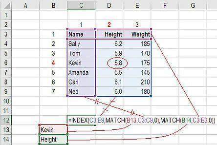
This image illustrates a two-way lookup. The formula uses one MATCH to find the row for "Kevin" and a second MATCH to find the column for "Height", returning the value 5.8 from the main data table.

Let's see this built from scratch.

The ULTIMATE Index Match Tutorial (5 Real-World Examples)

Now, watch the "Level 2" example from the same Kenji Explains video.

In this section, he extends the formula to handle two criteria: country and month. This demonstrates the INDEX(array, MATCH(), MATCH()) pattern for two-way lookups.

4. Handling Multiple Criteria

What if you need to look up a value based on three or more conditions that are all in different columns? For instance, find the "Total" for a "Product" sold by a specific "Company name". This is where INDEX-MATCH truly shines, though it requires a special type of formula known as an array formula.

The generic array formula is:
{=INDEX(return_range, MATCH(1, (criteria1=range1) * (criteria2=range2) * (criteria3=range3), 0))}

Important: This is an array formula. After typing it, you must press Ctrl + Shift + Enter instead of just Enter. Excel will automatically add curly braces {} around the formula.

The logic here is clever. Each (criteria=range) part creates an array of TRUE and FALSE values. When these arrays are multiplied, TRUE becomes 1 and FALSE becomes 0. The only row that gets a final value of 1 is the one where all conditions are met. The MATCH function then finds the position of this 1, giving INDEX the correct row number.

Excel INDEX MATCH with multiple criteria - formula examples

The article "Excel INDEX MATCH with multiple criteria" from Ablebits provides an excellent, detailed explanation of this technique.

First, read the section Excel INDEX MATCH with multiple criteria. This introduces the generic array formula and the critical instruction about using Ctrl + Shift + Enter. Next, study the formula example and explanation. Pay close attention to the "How this formula works" part, which breaks down how the multiplication of boolean arrays results in an array of 1s and 0s. This is the core concept to grasp.

This spreadsheet demonstrates the multiple criteria array formula. It looks for a record where the Company name is "Fabulous Book Store", the Contact is "John Wilson", and the Product is "Deep Sea Fishing" to return the corresponding Order Date.

Because array formulas can be fragile if other users aren't familiar with them, there is also a non-array alternative that is more robust. The Ablebits article you just reviewed also covers this clever technique in the section "Non-array INDEX MATCH formula with multiple criteria". It uses a second INDEX function to handle the array part internally, so you can just press Enter. This is a great professional habit to develop.

5. Looking Up Data Across Multiple Sheets

Finally, let's tackle the second part of our learning goal: looking up data across different worksheets. A common business scenario is having data split by division, region, or time period (e.g., a separate sheet for January, February, etc.). You need a way to build a summary report that can dynamically pull data from the correct sheet.

To do this, we combine INDEX-MATCH with another function: INDIRECT.

INDIRECT(ref_text): This function takes a text string that looks like a cell or range reference (e.g., "Sheet2!A1:B10") and turns it into an actual reference that Excel can use.

By constructing the sheet name as a text string, we can make our INDEX-MATCH formula dynamic. For example, if you have the name of the sheet you want to search (e.g., "Game Div") in cell B6, INDIRECT can build the reference for you.

Lookup Values Across Multiple Sheets in Excel (3 Methods)

This article from XelPlus, "How to Lookup Values Across Multiple Sheets in Excel," provides a complete guide. While it discusses several methods, we will focus on the INDEX-MATCH approach.

Start by reading the section How Do You Use INDEX MATCH to Lookup Data Across Sheets?. This section explains the best practice of converting your data ranges into named Excel Tables (Ctrl+T), which makes formulas cleaner and more manageable. Then, focus on the section How Do You Make INDEX MATCH Dynamic. This is the key part. It shows you how to use INDIRECT to refer to the table names dynamically. It also introduces SUBSTITUTE to handle spaces in sheet names, which is a common real-world challenge. The "Full Dynamic Formula" at the end puts it all together. For hands-on practice, the article provides a link to download the workbook, which is an excellent way to apply what you're learning.

Conclusion

In this lesson, you've taken a significant step in advancing your Excel skills from an average user to a data-savvy analyst. You've unlocked one of the most powerful formula combinations in Excel, which will serve you well in countless analytical tasks.

Here are the key takeaways:

INDEX-MATCH is a superior alternative to VLOOKUP due to its flexibility, robustness, and ability to look in any direction.
You can perform two-way lookups by using MATCH for both the row and column arguments of the INDEX function.
For lookups with multiple conditions, you can use an array formula that multiplies the criteria, or a more robust non-array version with a nested INDEX function.
To pull data from different sheets dynamically, you can combine INDEX-MATCH with the INDIRECT function to turn text into a valid range reference.

As an aspiring analyst, your job will be to find answers hidden in data. INDEX-MATCH is a primary tool for extracting the precise data points you need to begin your analysis.

In our next lesson, we will move from extracting individual data points to summarizing large datasets. You will learn how to create pivot tables, another cornerstone of data analysis in Excel, which allow you to quickly aggregate, group, and explore your data to uncover trends and insights.