Welcome to our next lesson on classical machine learning foundations. In our previous sessions, we explored probabilistic models like logistic regression and ensemble methods like Random Forests. Today, we'll delve into a powerful and elegant classification algorithm with a strong geometric intuition: the Support Vector Machine (SVM).
This lesson will equip you to explain the core principles of how SVMs work, from finding an optimal decision boundary in simple cases to handling complex, non-linear data. Mastering this is crucial for your interview, as SVMs represent a fundamental concept in machine learning, and interviewers often probe for a deep understanding of the "why" behind the algorithm, especially the famous "kernel trick."
We will start with the core idea of maximizing the margin between classes, then see how this idea is adapted for real-world, noisy data, and finally, we'll unravel the kernel trick that gives SVMs their power and flexibility.
The Core Idea: Maximizing the Margin
At its heart, an SVM is a classifier that seeks to find the best possible "hyperplane" that separates data points of different classes. For a 2D dataset, a hyperplane is simply a line. For 3D data, it's a plane, and so on.
However, for a given dataset, there might be many possible hyperplanes that can separate the classes. How does an SVM choose the best one? The core principle of SVM is to select the hyperplane that has the maximum margin. The margin can be thought of as the width of the "street" between the hyperplane and the closest data points from each class. By maximizing this margin, the model creates the largest possible separation between the classes, leading to better generalization on unseen data.
The data points that lie on the edges of this margin are called support vectors. They are the critical elements of the dataset because they alone "support" or define the position of the optimal hyperplane. If you were to move any other data point, the hyperplane wouldn't change. But if you move a support vector, the hyperplane will shift.
To build a solid foundation on these concepts, the following article and video provide excellent explanations.
Important Support Vector Machine (SVM) -Interview Questions [Updated 2025] - GeeksforGeeks
This GeeksforGeeks article is structured for interview preparation. It clearly defines the core concepts you'll need to articulate.
Please read the first three questions: What is the core idea, What are Support Vectors?, and What is margin in SVM. Focus on the clear, concise definitions provided.
Support Vector Machines: All you need to know!
This video from Intuitive Machine Learning provides a great visual introduction to the concepts of the hyperplane, margin, and support vectors.
Watch the introductory segment from the beginning until the end of the support vectors explanation. Pay attention to how the video visualizes the "street" and highlights the points that define its boundaries.
Dealing with Real-World Data: The Soft Margin
The maximal margin classifier we've just described (also called a hard margin SVM) works beautifully if the data is perfectly linearly separable. But what if it's not? What if there are outliers or the classes overlap slightly? A hard margin SVM would either fail to find a solution or create a very narrow margin that is highly sensitive to a few noisy points, leading to poor generalization.
This is where the soft margin SVM comes in. The soft margin approach allows for a more flexible model that can tolerate some misclassifications. It aims to find a balance between two competing goals:
- Making the margin as wide as possible.
- Minimizing the number of "margin violations" (points that are on the wrong side of the margin or even the wrong side of the hyperplane).
This trade-off is controlled by a crucial hyperparameter, typically denoted as C.
- A small C value creates a wide margin but allows more margin violations. This can lead to a simpler model that may generalize better (higher bias, lower variance).
- A large C value creates a narrow margin and penalizes margin violations heavily. The model will try to classify every training example correctly, which can lead to a more complex decision boundary that might overfit the training data (lower bias, higher variance).
The mechanism for allowing these violations is the use of slack variables (often denoted by the Greek letter zeta, ). Each data point gets a slack variable, which is zero if the point is correctly classified and outside the margin, and positive if it violates the margin. The hyperparameter C then acts as a regularization parameter that controls the total penalty assigned to these slack variables.
Machine Learning Algorithms Explained: Support Vector ...
The StrataScratch article provides a clear, step-by-step evolution from the hard margin concept to the soft margin.
First, read the section on the Maximal Margin Classifier to understand its limitations. Then, read the section on Soft Margin, which explains how allowing misclassifications relates to the bias-variance tradeoff. Finally, in the section "Support Vector Machine Under the Hood," focus on the part that explains the role of the C hyperparameter.
The Kernel Trick: Conquering Non-Linearity
We've seen how soft margins can handle overlapping classes, but what if the decision boundary is fundamentally non-linear? For example, what if one class is a circle of points surrounded by another class? No straight line can separate them.
This is where SVMs truly shine, thanks to the kernel trick. The core idea is simple: if the data is not linearly separable in its current dimension, we can project it into a higher-dimensional space where it does become linearly separable.

The problem with this approach is that explicitly calculating the coordinates of each data point in a new, potentially very high-dimensional space can be computationally expensive or even impossible.
This is where the "trick" comes in. The mathematical formulation of the SVM (specifically, the "dual form" which you may encounter in more advanced texts) shows that the algorithm only needs the dot product of the feature vectors, not their actual coordinates. The kernel trick leverages this by using a kernel function, which is a function that takes two data points in the original space and directly computes what their dot product would be in the higher-dimensional space, without ever performing the explicit transformation.
This is a computationally brilliant shortcut. It allows us to get all the benefits of working in a high-dimensional feature space without paying the computational price.
The following video provides one of the clearest explanations of this powerful concept available.
SVM Kernels : Data Science Concepts
This video by ritvikmath masterfully builds the intuition for why the kernel trick is both necessary and brilliant.
Please watch the entire video. It progresses through several key stages: A motivating example shows why we need to go to a higher dimension. The inefficiency of explicit transformation is explained, setting up the need for a "trick." A concrete example shows how a kernel function can reproduce the high-dimensional dot product using only low-dimensional data. The final segment summarizes the concept of a kernel function.
Common Kernels and Their Effect
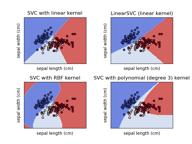
With the kernel trick, our choice of kernel function determines the shape of the decision boundary. Here are the most common ones:
- Linear Kernel: No transformation is applied. This is equivalent to a standard soft-margin SVM and is used when the data is already mostly linearly separable.
- Polynomial Kernel: Creates decision boundaries that are polynomials of a certain degree. The key hyperparameter is the
degree. Higher degrees can model more complex boundaries but risk overfitting. - Radial Basis Function (RBF) Kernel: This is the most popular and generally the most effective kernel. It can create highly complex, non-linear boundaries. It maps the data into an infinite-dimensional space. Its key hyperparameter is
gamma.gammacan be thought of as the inverse of the radius of influence of samples selected by the model as support vectors.- A low
gammameans a large radius of influence, so the decision boundary is smoother and less complex. - A high
gammameans a small radius of influence, so the model is more influenced by points close to the boundary, resulting in a more complex, "wiggly" boundary that can easily overfit.
The image below, from the scikit-learn documentation, shows the effect of different kernels on the same dataset.
To solidify your understanding of these kernels and their hyperparameters, please refer back to the resources we've used.
Machine Learning Algorithms Explained: Support Vector ...
The StrataScratch article provides clear descriptions of the most common kernels.
Read the section explaining the intuition of SVMs and kernels, and then read the brief descriptions of the Polynomial Kernel and the RBF Kernel.
Conclusion
In this lesson, we've dissected the Support Vector Machine algorithm, a cornerstone of classical machine learning. You are now prepared to discuss its mechanisms with the depth and clarity required for a technical interview.
Key Takeaways:
- Core Principle: SVMs work by finding an optimal hyperplane that maximizes the margin between classes, leading to better generalization.
- Support Vectors: These are the data points lying on the margin that uniquely define the hyperplane's position.
- Soft Margin & 'C': For real-world data, the soft margin SVM allows for some misclassifications by using slack variables. The hyperparameter C controls the trade-off between maximizing the margin and minimizing these classification errors.
- The Kernel Trick: This is the elegant solution for non-linear data. It uses a kernel function (e.g., Polynomial, RBF) to efficiently compute dot products in a higher-dimensional space, allowing the SVM to find a linear separator there without the computational cost of an explicit transformation.
- Hyperparameters: The choice of
kerneland its associated parameters (degreefor polynomial,gammafor RBF) along withCare critical for tuning an SVM's performance.
In our next lesson, we will begin our dive into Feature Engineering and Preprocessing. We'll start with essential techniques like feature scaling and normalization. This is a perfect follow-up, as the performance of SVMs is highly sensitive to the scale of the input features, a practical consideration you'll need to be aware of when applying them.