Welcome to the second module of our course. As we move from the theoretical foundations of classical models into the practicalities of building them, we'll start with one of the most fundamental and impactful steps in any machine learning pipeline: feature engineering and preprocessing.
In our last lesson on Support Vector Machines, we concluded by noting that their performance is highly sensitive to the scale of input features. This is true for many algorithms. Today, we'll address this directly by learning how to apply feature scaling, normalization, and log transformations. Understanding these techniques is not just about improving model accuracy; it's a core competency that interviewers expect you to master, as it demonstrates your grasp of how data characteristics interact with algorithm mechanics.
This lesson will equip you to:
- Explain why scaling and transformations are necessary.
- Choose the appropriate technique based on the data's distribution and the presence of outliers.
- Apply these methods using common Python libraries.
Why Do We Need to Scale and Transform Data?
Machine learning models, at their core, are mathematical functions. If you feed them features with vastly different scales—for instance, a person's age (e.g., 20-70) and their annual income (e.g., $30,000 - $1,000,000)—the feature with the larger range (income) will numerically dominate the calculations. This can cause significant problems.
Many algorithms are susceptible to this issue:
- Distance-based algorithms: As we saw with SVMs, algorithms like k-Nearest Neighbors (KNN) and clustering methods (e.g., K-Means) rely on calculating distances between data points. An unscaled feature with a large range will disproportionately influence this distance metric, effectively making other features irrelevant.
- Gradient-based algorithms: Models trained with gradient descent, such as linear/logistic regression and neural networks, often converge much faster and more reliably when features are on a similar scale. This is because scaling can result in a more spherical or less elliptical cost function landscape, making it easier for the optimizer to find the minimum.
On the other hand, some models are largely immune to feature scaling. Tree-based models like Decision Trees, Random Forests, and Gradient Boosting are not affected because their splitting decisions are based on individual features, not on distances between them. Knowing this distinction is a key piece of practical ML knowledge.
For a great visual intuition of why unscaled features can be problematic, the following video provides an excellent demonstration using Euclidean distance.
What is Feature Scaling? | Standardization | Normalization | Data Preprocessing in Python
This video from Six Sigma Pro SMART clearly illustrates how a feature with a large magnitude can dominate a distance calculation, leading to skewed interpretations.
Watch the section from the beginning to about the end of the Euclidean distance example. Pay close attention to how changing the units of the 'sales' feature completely alters its contribution to the overall distance.
A Quick Note on Terminology
Before we dive into the methods, it's helpful to clarify some terms that are often used interchangeably, which can cause confusion.
- Scaling: Generally refers to changing the range of your data without changing the shape of its distribution. The relative positions of data points are preserved.
- Normalization: This term is ambiguous. In many contexts, it's used as a synonym for Min-Max scaling (scaling to a [0, 1] range). In a stricter statistical sense, it means transforming your data to follow a normal (Gaussian) distribution.
- Transformation: A broader term for any mathematical function applied to the data. This can include scaling, but also operations that change the data's distribution, like log or Box-Cox transformations.
For clarity in this lesson, we will use "scaling" to refer to range adjustments (like Standardization and Min-Max) and "transformation" for operations that alter the distribution's shape (like Log Transform).

Scaling Techniques: Adjusting the Range
Let's explore the most common methods for scaling data. The following article provides excellent code examples and context for each.
Scaling Numerical Data, Explained: A Visual Guide with ...
This article from Towards Data Science gives a concise overview of why and when to scale data, which serves as a great introduction to the specific techniques we'll cover.
Please read from the beginning, including the sections Understanding Which Data Needs Transformation and Why Scale Your Data?. This will reinforce the concepts we just discussed.
1. Standardization (Z-Score Scaling)
This is arguably the most common and robust scaling technique. It transforms your data to have a mean of 0 and a standard deviation of 1.
The formula for each data point is:
where is the mean of the feature and is its standard deviation.
- When to use: It's a great default choice, especially for algorithms that assume data is centered around zero (like SVMs, logistic regression, and neural networks). It works well when your data is approximately normally distributed.
- Caveat: Since the mean and standard deviation are used in the formula, standardization can be affected by extreme outliers, which can pull the mean and inflate the standard deviation.
For a clear explanation and scikit-learn implementation, this video is very helpful.
Normalization Vs. Standardization (Feature Scaling in Machine Learning)
This video from Prof. Ryan Ahmed walks through the concept of standardization and shows how to implement it using StandardScaler.
Watch the segment on standardization, from the beginning of the standardization section until the comparison. Pay attention to the resulting mean (0) and standard deviation (1) in the statistical summary.
2. Min-Max Scaling (Often called Normalization)
This technique scales your data to a fixed range, typically [0, 1].
The formula for each data point is:
where and are the minimum and maximum values of the feature.
- When to use: It's useful when you need your data within a specific bounded interval. For example, image data where pixel values (0-255) are scaled to [0, 1] for input into a neural network. It's also easy to interpret.
- Caveat: It is highly sensitive to outliers. A single outlier with a very high or low value will become the new
maxormin, squishing all other data points into a very small part of the [0, 1] range.
The video you just watched also covers Min-Max scaling.
Normalization Vs. Standardization (Feature Scaling in Machine Learning)
This segment from Prof. Ryan Ahmed's video explains Min-Max scaling and its implementation with MinMaxScaler.
Focus on the first part of the video, from the normalization section. Notice how the minimum value becomes 0 and the maximum becomes 1 after the transformation.
3. Robust Scaling
This technique is designed to be, as the name suggests, robust to outliers. Instead of using the mean/standard deviation or min/max, it uses statistics based on the median and the interquartile range (IQR). The IQR is the range between the 1st quartile (25th percentile) and the 3rd quartile (75th percentile).
The formula for each data point is:
- When to use: This is the preferred method when your dataset has significant outliers. In a fintech context, dealing with transactional data, income, or market data, outliers are common, making Robust Scaling a very important tool in your toolkit.
- Caveat: It does not scale the data to a specific, bounded range like Min-Max scaling.
Scaling Numerical Data, Explained: A Visual Guide with ...
Let's return to the Towards Data Science article to see how Robust Scaling is implemented.
Read Method 3: Robust Scaling. The example application to 'Humidity' with potential outliers is a good one.
Transformation: Changing the Shape
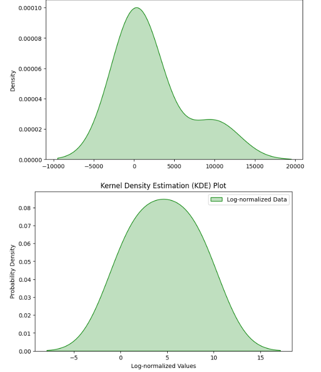
Sometimes, the problem isn't the range of the data, but its distribution. Many real-world variables, particularly in finance (like income, wealth, transaction sizes), follow a right-skewed or power-law distribution. This means most values are clustered at the low end, with a long tail of infrequent, high-value observations. Such distributions can violate the assumptions of many linear models.
Log Transformation
The most common way to handle right-skewed data is to apply a logarithmic transformation. This compresses the range of the higher values more than it compresses the range of the lower values, pulling the long tail in and making the distribution more symmetric and "normal-like".
The formula is simply . Since is undefined, if your data contains zeros, you would typically use .
Numerical data: Normalization | Machine Learning | Google for Developers
This Google Developers article provides a great explanation for why log scaling is useful in the context of power-law distributions.
Please read the section on Log scaling. The examples of movie ratings and book sales clearly illustrate the kind of distributions where this technique is most effective.
Summary and Practical Advice for Interviews
Being able to articulate the trade-offs between these methods is crucial for an interview. Here's a summary table based on the Google ML Crash Course resource.
| Technique | Formula | When to Use |
|---|---|---|
| Min-Max Scaling | When you need data in a bounded range [0, 1]. Best for uniformly distributed data with no significant outliers. | |
| Standardization | General-purpose, default choice. Best for data that is approximately normally distributed. | |
| Robust Scaling | When your data contains significant outliers. Very common in real-world datasets, especially fintech. | |
| Log Transform | To handle right-skewed data and make its distribution more symmetric/normal. This is a transformation, not scaling. |
A Critical Implementation Note: When you preprocess your data, you must calculate the scaling parameters (e.g., mean and standard deviation for Standardization) from the training set only. You then use these same parameters to transform both your validation and test sets. If you were to fit on the test set, you would be "leaking" information from the future into your training process, which invalidates your model evaluation. In scikit-learn, this means you call fit_transform() on the training data, but only transform() on the test/validation data.
Conclusion
You've now covered the essential techniques for preparing numerical data for modeling. Raw data is rarely in a state that's optimal for machine learning algorithms, and applying the correct scaling or transformation is a critical step that directly impacts model performance, training time, and reliability.
Key Takeaways:
- Why: We scale data to prevent features with large ranges from dominating distance or gradient-based calculations. We transform data to make its distribution more suitable for certain model assumptions.
- Standardization (
StandardScaler): The go-to for centering data (mean=0, std=1). Good for normally-distributed data. - Min-Max Scaling (
MinMaxScaler): Use when you need data in a strict [0, 1] range. Highly sensitive to outliers. - Robust Scaling (
RobustScaler): The best choice when dealing with data containing significant outliers, as it uses the median and IQR. - Log Transformation: Not a scaling method, but a transformation to handle right-skewed data and make it more symmetric.
In our next lesson, we will continue our journey through data preprocessing by tackling another ubiquitous problem: missing data. We'll explore different strategies for imputing missing values and discuss the trade-offs involved with each approach.