Introduction
Welcome to the fourth lesson in our module on parallel architectures. In our previous lessons, we focused on shared-memory systems, where multiple processors access a common memory space. We saw how protocols like MESI are crucial for maintaining cache coherence in such systems. This model is like a team of engineers working on a single, large whiteboard—everyone sees the same information, and the hardware ensures the whiteboard is kept consistent.
Today, we pivot to a fundamentally different paradigm: distributed-memory architectures. In this model, there is no shared whiteboard. Instead, each engineer has their own private notebook and communicates by passing notes. This lesson will describe these architectures and explain the critical role of the interconnection networks that act as the "postal service" for these notes. This forms the architectural basis for many of the world's largest supercomputers.
From Shared to Distributed Memory
In a shared-memory system, communication between cores is implicit. A write to a memory location by one core is made visible to others through hardware coherence mechanisms.
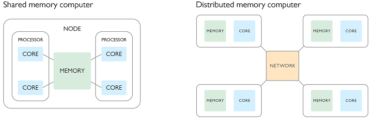
In a distributed-memory system, communication is explicit. Each processor, or node, has its own private memory. A processor cannot directly access another processor's memory. To share data, one processor must explicitly package the data into a message and send it to another processor, which must explicitly receive it.
The image below provides a clear visual distinction between these two models.
To see a narrated explanation of this distinction, let's watch a brief segment of the following video.
Shared and Distributed Memory architectures
This video revisits the shared-memory concept and introduces the distributed-memory architecture, highlighting the fundamental difference in how processors communicate.
Watch from the beginning to 03:25. Focus on how remote memory access differs between the two models. In shared memory, it's a simple load/store instruction. In distributed memory, it requires an explicit I/O operation across the network, which is a more involved and expensive process.
As the video explains, accessing remote data in a distributed system is not a single instruction but a coordinated procedure of sending and receiving messages. This is the foundation of the message-passing programming paradigm.
The Message-Passing Model
Programs for distributed-memory systems are typically written using the message-passing model. The de facto standard library for this is the Message Passing Interface (MPI). While we will dive deep into MPI programming in a later module, understanding its core concepts is essential for grasping the architecture.
In the MPI model:
- A program is launched as a set of independent processes.
- Each process is assigned a unique integer ID called its rank.
- All processes belong to a communication group called a communicator. The default,
MPI_COMM_WORLD, includes all processes. - Processes communicate by calling functions like
MPI_SendandMPI_Recv.
Introduction to Parallel Computing | ARC4CFD
This article uses a great analogy of students in separate rooms to explain the message-passing concept. It also introduces different types of communication.
Please read the following sections: Start at 'Distributed memory architecture & distributed parallelism'. Read through to the end of the sub-section 'Interprocessor communication: message passing'. This part covers the core analogy, blocking vs. non-blocking communication, and different communication patterns (point-to-point vs. collective). Then, skip to the section 'MPI in Python' and read its introduction to see how concepts like rank and communicator are defined.
As you read, note the two main advantages of the distributed-memory model:
- No data corruption risk: Since memory is private, one process cannot accidentally overwrite another's data.
- Memory scalability: The total system memory scales with the number of processors, unlike a shared-memory system, which is limited by a single physical memory unit.
The Role of the Interconnection Network
The collection of nodes in a distributed-memory system is often called a cluster. The performance of such a system is heavily dependent on the communication fabric that connects the nodes: the interconnection network. This network consists of:
- Endpoints: The processors/nodes themselves.
- Links: The physical wires or optical fibers that carry data.
- Switches: Devices that route messages from an incoming link to the correct outgoing link, directing them toward their destination.
The way these components are arranged is called the network topology. The topology determines the performance, cost, and scalability of the entire parallel machine.
Lecture notes: Interconnection networks
The following lecture notes provide a formal introduction to interconnection networks and their key characteristics.
Read the 'Introduction' (Section 1) and the section 'Network characteristics' (Section 2.1). Focus on understanding the definitions of direct vs. indirect networks and the key performance metrics: diameter and bisection bandwidth.
Key Network Performance Metrics
As outlined in the notes, we evaluate network topologies using a few key metrics:
- Diameter: The longest shortest path between any two nodes in the network. This represents the worst-case latency for sending a message, assuming no network congestion. A smaller diameter is better.
- Bisection Bandwidth: The minimum number of links you must cut to divide the network into two equal halves. This measures the network's communication bottleneck and is a crucial indicator of its ability to handle global communication patterns where many nodes communicate simultaneously. A larger bisection bandwidth is better.

- Degree: The number of links connected to a single node or switch. This is a primary indicator of the network's hardware cost and complexity.
An ideal network has a low diameter, high bisection bandwidth, and a low degree. In practice, there are always trade-offs.
Common Network Topologies
Let's explore some common topologies and their trade-offs. These are categorized as either direct networks, where processors are part of the network fabric, or indirect networks, where processors connect to a separate network of switches.
Lecture notes: Interconnection networks
Now, let's examine specific network topologies using the same lecture notes.
Read the sections 'Static networks' (Section 2.2) and 'Dynamic networks' (Section 3). Pay attention to the properties (degree, diameter, bisection bandwidth) and the pros and cons of each topology: Static (Direct): Ring, 2D/3D Mesh, and 2D/3D Torus. Dynamic (Indirect): Fat-Tree.
Here is a summary of the key topologies you just read about:
| Topology | Type | Degree (Cost) | Diameter (Latency) | Bisection Bandwidth (Throughput) | Comments |
|---|---|---|---|---|---|
| Ring | Direct | Low (2) | Poor (proportional to N) | Poor (constant) | Simple and cheap, but doesn't scale well. The communication pattern in the "MPI Basics" video LINK creates a logical ring. |
| 2D Mesh | Direct | Medium (4) | Moderate (proportional to √N) | Moderate (proportional to √N) | Good for problems with local communication, like grid-based physics simulations. Edges are a drawback. |
| 2D Torus | Direct | Medium (4) | Good (half of mesh) | Good (double mesh) | A mesh with "wraparound" connections. Better performance than a mesh for a small increase in cost. |
| Fat-Tree | Indirect | Varies | Excellent (constant, low) | Excellent (proportional to N) | Highly scalable and provides high bandwidth for arbitrary communication. Very common in modern data centers and supercomputers. |
Your engineering background gives you a good intuition for grid-based problems. A 2D Mesh topology is a natural fit for simulating a 2D physical space, as each node can directly communicate with its north, south, east, and west neighbors, minimizing communication distances for local interactions.
The Fat-Tree is particularly important. Its design ensures that bandwidth does not decrease as you move up the hierarchy toward the "root," avoiding the bottleneck that a simple tree structure would create. This makes it excellent for all-purpose clusters where communication patterns are not predictable.
Conclusion
In this lesson, we have moved from the tightly-coupled world of shared memory to the scalable but more complex realm of distributed memory.
Key Takeaways:
- Distributed-memory architectures consist of independent nodes, each with its own private memory. Communication is explicit, achieved by sending and receiving messages.
- The Message Passing Interface (MPI) is the standard programming model for these systems.
- The interconnection network is the physical fabric connecting the nodes, and its topology is critical to the system's performance and scalability.
- Network performance is evaluated using metrics like diameter (latency) and bisection bandwidth (throughput).
- Common topologies like Ring, Mesh, and Torus are direct networks with different cost-performance trade-offs.
- The Fat-Tree is a highly scalable indirect network topology used in many modern high-performance clusters because it avoids communication bottlenecks.
Preview of the Next Lesson
We have now examined two of the main parallel architectures: shared-memory and distributed-memory systems. In our next lesson, we will explore a third, highly influential architecture: the Graphics Processing Unit (GPU). We will describe its unique structure, including streaming multiprocessors, warps, and its specialized memory hierarchy. You will see how GPUs represent a massively parallel architecture that combines elements of both shared and distributed models to achieve incredible computational throughput for specific types of problems.