Hello. In the previous lesson, you examined whether a subsidy’s eligibility and award rules fit its public purpose. Fair-looking rules leave a separate question: did the subsidy produce a benefit that would not otherwise have occurred? This lesson develops an estimate from observed outcomes and a defensible picture of what would have happened without support. Allow about 40 minutes, including the readings and short video.
The missing outcome
Suppose a grant pays factories to replace high-emission heaters. Seventy qualifying heaters are replaced during the grant year. That is an observed outcome, but it is not yet the grant’s additional benefit: some factories might have replaced their heaters anyway.
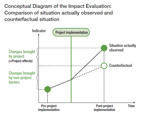
The outcome without the grant is called the counterfactual or reference case. It cannot be observed for the same factories in the same year. The task is to estimate it credibly, then compare like with like:
The diagram below separates the observed result from the counterfactual at the same point in time. Notice that the counterfactual rises above the pre-project level: other forces can produce improvement even without the project.
Read the short explanation from What Works Growth. Its distinction between activity that occurred and activity caused by the policy applies directly to a subsidy.
Understanding additionality and deadweight - What Works Growth
What Works Growth explains additionality, deadweight, and why a comparison is needed. Read it for the meaning of the estimate, rather than for a calculation method.
In “What is additionality?”, read from the opening definition through the examples at the end of that subsection. Continue through “What is deadweight?” to the closing qualification. Finally, under “What to consider when thinking about additionality and deadweight?”, read the comparison explanation, stopping before the paragraph beginning “Often, we might want a feeling”.
Deadweight refers to supported activity that would have happened anyway. If the grant-year total is 70 replacements and the credible no-grant estimate is 50, the estimate is 20 additional replacements. The other 50 are not necessarily identifiable individual heaters; 50 is an estimate of how much activity the group would have undertaken without the grant.
The counterfactual is also different from the baseline, which describes the position before the intervention. Last year’s replacement rate may be useful evidence, but it need not be this year’s no-grant rate. Equipment may be aging, prices may change, and other rules may already require upgrades.
The Additionality Guide develops this distinction. Its account of a reference case is useful when judging whether a supplied “without subsidy” number has an evidential basis.
The Additionality Guide explains why a reference case must account for likely change over time. Read its discussion of the baseline and the evidence used to construct a no-intervention estimate.
In Chapter 3, “The reference case (assessing deadweight),” read Sections 3.1 “Overview,” 3.2 “Measuring the baseline position,” and 3.3 “Assessing the reference case” on printed pp. 17–18. Begin with the reference-case discussion. Stop after the warning that the baseline and reference case should not simply be assumed equal, before the paragraph beginning “When assessing the additional impacts of an intervention.” Focus on the evidence and assumptions needed to justify a “do minimum” case.
Building the estimate from comparison data
A tempting calculation is to subtract last year’s replacements from this year’s. But if replacements were rising across the industry, that calculation would credit the grant for an existing trend. Comparing grant recipients with nonrecipients only after the grant is also risky: the groups may have differed before support began.
The World Bank Group’s short video shows both problems and explains why a lottery can sometimes create a stronger comparison.
“What is Impact Evaluation?” from the World Bank Group explains why an observed improvement alone does not establish a program’s effect.
Watch two weak comparisons for the problems with before-and-after figures and with participants who select themselves into a program. Then watch the lottery example for how assigning available places by chance can make groups more comparable on average.
Now consider fictional data for the heater grant. The measure is the number of qualifying replacements per 100 facilities in each one-year period. The grant begins before the second period.
| Facilities | Year before grant | Grant year | Change |
|---|---|---|---|
| Facilities receiving the grant | 20 | 70 | 50 |
| Comparable facilities without the grant | 25 | 55 | 30 |
The subsidized group made 70 replacements in the grant year—50 more than in its previous year. But replacements also increased by 30 in the comparison group. If that group’s increase is a credible estimate of the trend the subsidized facilities would have experienced without support, the subsidized group’s counterfactual is its earlier 20 plus that trend of 30: 50 replacements.
The resulting estimate is:
per 100 subsidized facilities in that year. Equivalently, the subsidized group’s increase of 50 exceeds the comparison group’s increase of 30 by 20. Using changes rather than simply subtracting the two grant-year totals matters here: the groups started at different levels.
This calculation is only as persuasive as its comparison assumption. Facilities with and without grants should face reasonably similar influences on replacement decisions. Earlier trends, equipment age, firm size, energy prices, and other applicable policies would help assess that claim. If grants went mainly to facilities already planning an unusual wave of replacements, the comparison group’s ordinary trend could understate what recipients would have done anyway. Conversely, if the grant caused unsubsidized firms to postpone upgrades, their observed trend would be a poor no-grant benchmark. The arithmetic is exact for the supplied figures; the causal interpretation remains conditional.
What the number supports—and what it does not
The estimate of 20 concerns annual heater replacements per 100 subsidized facilities. It does not by itself measure emissions avoided, how long the new equipment remains in use, or whether the grant merely brought forward replacements that would occur next year. The policy objective determines which outcome ultimately matters. Replacement counts are a useful intermediate measure if cleaner equipment is the goal, but measured emissions would speak more directly to that goal.
Suppose the 100 subsidized facilities received 400,000 in total grants during the year. On the central estimate, public spending was 20,000 per additional replacement:
That is a cost per additional measured replacement, not proof that the policy delivered value exceeding its cost. Assessing that would also require evidence about emissions, other benefits, costs imposed elsewhere, and possible alternative uses of the funds.
It is helpful to show how dependent the result is on the counterfactual. If a defensible estimate of the no-grant trend were anywhere from 20 to 40 replacements, rather than exactly 30, the no-grant outcome for recipients would range from 40 to 60. The estimated additional replacements would consequently range from 30 down to 10. This range does not establish that either endpoint is correct; it makes the consequence of uncertainty visible.
At the central estimate, 50 of the 70 grant-year replacements would have occurred anyway in aggregate—about 71% of the observed replacement count. Do not automatically call 71% of the grant money wasted. Payments may differ among projects, and a grant could also improve the timing or quality of replacements. Equally, paying for many replacements that would have occurred anyway is a reason to examine whether a more targeted design could achieve the same public purpose at lower cost.
Finally, additionality and favoritism are different tests. A grant with little additional effect may be poorly designed without being politically connected. A grant that produces a substantial effect may still have been awarded through preferential rules. The prior lesson assessed access and award decisions; this estimate assesses what the support appears to have changed.
Conclusion
A subsidy’s additional benefit is the difference between an observed outcome and a credible estimate of that same outcome without the subsidy. A pre-grant baseline is evidence for that estimate, not automatically the counterfactual. In the fictional heater data, accounting for the comparison group’s trend yields an estimate of 20 additional annual replacements per 100 subsidized facilities, rather than the observed increase of 50.
State the outcome, period, comparison assumption, and uncertainty alongside any number. That makes the estimate useful without claiming more than the evidence supports. The next lesson turns from subsidies to public tenders, where specifications and award procedures can create warning signs of favoritism without proving it.