Understanding the Bias-Variance Tradeoff

Understanding Bias and Variance Intuitively

At a high level, the error a model makes can be broken down into three components: bias, variance, and irreducible error. We can't do anything about irreducible error—it's the inherent noise in any real-world dataset. Our focus, therefore, is on managing bias and variance.

To build a strong intuition for these two concepts, let's start with an excellent video from StatQuest. It uses a simple, clear example to illustrate what happens when a model has high bias versus when it has high variance.

The video introduces the idea of a simple model (the straight line) being too rigid and a complex model (the squiggly line) being too flexible.

• Bias is the error from overly simplistic assumptions in the learning algorithm. A high-bias model fails to capture the underlying trend in the data. Think of the straight line failing to model the curve in the data—this is underfitting.
• Variance is the error from being too sensitive to small fluctuations in the training data. A high-variance model fits the training data, including its noise, too closely. Think of the squiggly line that perfectly fits the training points but performs poorly on the test points—this is overfitting.

The bullseye analogy is a classic way to visualize this. Imagine the center of the target is the true value we want to predict. Each blue dot is a prediction made by a model trained on a different subset of our data.

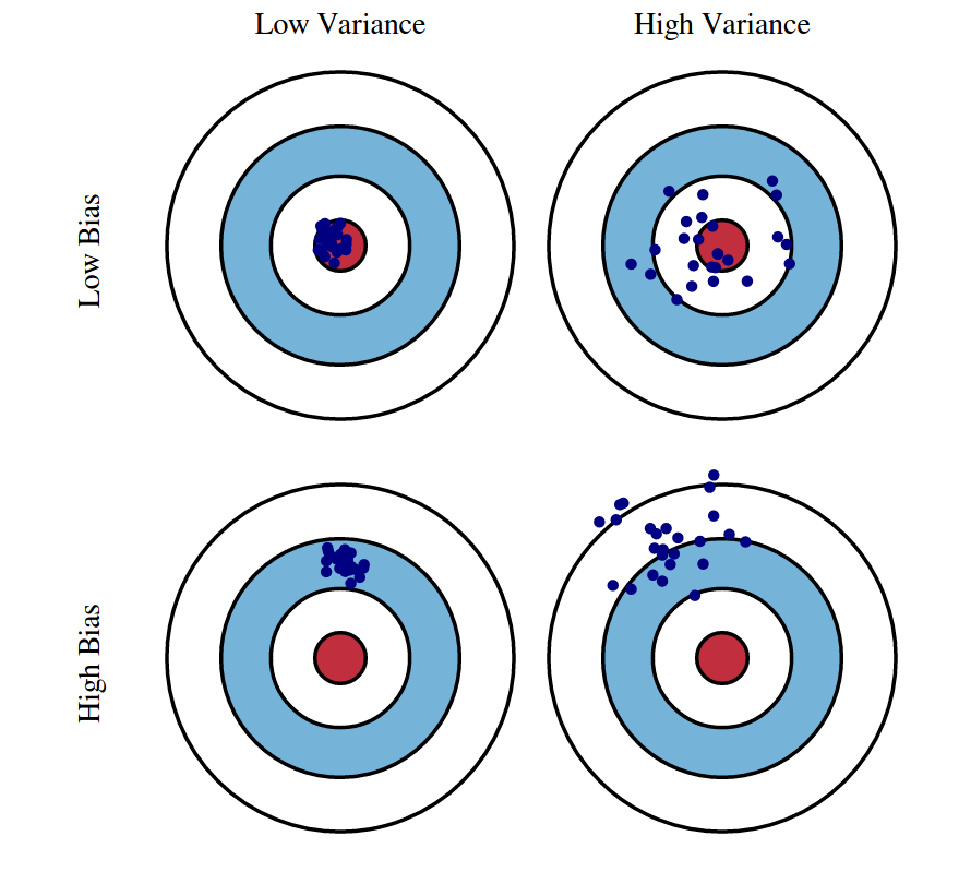
• Low Bias, Low Variance (Top-Left): The ideal scenario. Predictions are accurate (centered on the bullseye) and consistent (tightly clustered).
• Low Bias, High Variance (Top-Right): The model's predictions are, on average, correct, but they are scattered. This is overfitting; the model is sensitive to the specific training data it saw.
• High Bias, Low Variance (Bottom-Left): The model's predictions are consistent but systematically wrong. This is underfitting; the model is too simple to capture the true relationship.
• High Bias, High Variance (Bottom-Right): The worst of both worlds. Predictions are inaccurate and inconsistent.

The Tradeoff and Model Complexity

The key insight is that bias and variance are often in tension. As we increase a model's complexity to reduce bias, we tend to increase its variance, and vice-versa. This relationship is central to model selection.

Let's break down the graph above:

1. On the left (Low Complexity): Simple models (like linear regression for a complex problem) have high bias and low variance. They underfit the data, resulting in high error on both the training and test sets.
2. On the right (High Complexity): Complex models (like a very deep decision tree or a high-degree polynomial) have low bias and high variance. They can "memorize" the training data, leading to very low training error, but they fail to generalize to the test set. The high test error is a sign of overfitting.
3. In the middle (The "Sweet Spot"): The optimal model complexity is where the sum of bias and variance is minimized. This corresponds to the lowest point on the test error curve, achieving the best possible performance on unseen data.

The Stanford Online video featuring Trevor Hastie provides a more formal look at this phenomenon and the mathematical decomposition of error.

As the video explains, the expected test error for a given prediction can be decomposed like this:

Your goal as an engineer is to select a model and tune its complexity to find the sweet spot that minimizes the sum of bias and variance.

Practical Implications: Diagnosis and Correction

Recognizing whether your model is suffering from high bias or high variance is a critical diagnostic skill. The following article provides an excellent summary of the differences and, more importantly, practical strategies for addressing each problem.

Let's distill the key strategies from the reading:

To Fix High Bias (Underfitting):
Your model is too simple. You need to increase its ability to learn the patterns.

• Increase Model Complexity: Switch from a simple algorithm to a more powerful one (e.g., from linear regression to a random forest or neural network).
• Add More Features: Provide the model with more information by engineering new features or adding new data sources.
• Decrease Regularization: Regularization techniques are designed to prevent overfitting by penalizing complexity. If your model is already underfitting, you may be regularizing too much.

To Fix High Variance (Overfitting):
Your model is too complex or has learned the noise in your data. You need to simplify it or help it generalize better.

• Get More Training Data: This is often the most effective way to combat overfitting. More data helps the model learn the true signal instead of the noise.
• Simplify the Model: Use a less complex algorithm, or reduce the complexity of your current one (e.g., prune a decision tree, reduce layers/neurons in a neural network).
• Use Regularization: Apply techniques like L1/L2 regularization, dropout, or early stopping to penalize complexity and discourage the model from fitting the noise.
• Feature Selection: Remove irrelevant or noisy features to reduce the complexity of the problem.

Conclusion

In this lesson, we've explored the fundamental tension between bias and variance that lies at the heart of model development.

Key Takeaways:

• Bias represents a model's systematic error due to overly simple assumptions, leading to underfitting.
• Variance represents a model's sensitivity to the specific training data, leading to overfitting.
• There is a tradeoff: increasing model complexity typically decreases bias but increases variance.
• The goal of model selection is to find the "sweet spot" of complexity that minimizes the total error on unseen data.
• We can diagnose whether a model suffers from high bias or high variance and apply specific strategies to correct it.

Understanding this tradeoff is the "why" behind many practices in MLOps. When we tune hyperparameters or select a model architecture, we are fundamentally trying to navigate this tradeoff.

But how do we practically measure the test error to find this sweet spot without "contaminating" our final evaluation? We can't use the test set during the development process. This conundrum leads directly to our next topic: the crucial methodology of splitting data into training, validation, and test sets, which provides a principled way to estimate a model's generalization ability and tune its complexity.