Welcome to the final lesson in our module on the foundations of financial modeling. In our previous sessions, you've built a complete, dynamically linked three-statement model and, most recently, fortified it with automated validation checks. You now have a trustworthy tool that correctly reflects the fundamental accounting equation.
Today, we'll put that tool to its most powerful use: exploring the future. This lesson is dedicated to scenario analysis, a technique central to your goal of mastering strategic foresight. We will move beyond a single forecast and learn how to model a range of potential outcomes—specifically, a base, bull, and bear case. You will learn to identify key business drivers, define different assumptions for them, and structure your Python code to run and compare these scenarios, transforming your model from a static calculator into a dynamic decision-making instrument.
Why a Single Forecast is Not Enough
A financial forecast is built on assumptions, and assumptions are inherently uncertain. A single-point forecast, while useful, presents a single version of the future and fails to capture the range of possibilities. Strategic planning, risk management, and valuation all require a more nuanced view.
Scenario analysis addresses this by creating several distinct, internally consistent stories about the future.
Scenario & Sensitivity Modeling in Excel | FMVA® Course Preview
This video from the Corporate Finance Institute provides an excellent conceptual introduction to scenario and sensitivity modeling.
Please watch the first few minutes to understand the core ideas: Introduction : The speaker explains why a single valuation number is insufficient and introduces the concepts of scenario and sensitivity analysis. Compare and Contrast : Pay close attention to this section, which clearly defines scenario analysis (changing multiple inputs for discrete "cases") versus sensitivity analysis (changing one input at a time). Why Perform Scenario Analysis? : This part connects the technique directly to business planning and valuation, which should align well with your experience in corporate strategy.
As the video highlights, we typically model three main scenarios:
- Base Case: The most likely outcome, based on your best estimates.
- Bull (or Upside) Case: An optimistic scenario where key drivers perform better than expected.
- Bear (or Downside) Case: A pessimistic scenario where key drivers underperform.
The output of such an analysis often looks like a table comparing these different futures, allowing for clear strategic discussion.

Implementing Scenarios in Python
In a spreadsheet environment like Excel, analysts often use a "switch" or a dropdown menu to toggle between scenarios. In Python, we can achieve a more robust and scalable solution by structuring our assumptions and model logic thoughtfully. The process involves three main steps:
- Isolate Assumptions: Define the assumptions for each scenario in a separate data structure, like a dictionary.
- Encapsulate Model Logic: Wrap the entire financial model calculation process into a single, reusable function that accepts an assumptions dictionary as an argument.
- Iterate and Analyze: Loop through the different scenario assumptions, run the model for each, and collect the results for comparison.
Let's apply this to the model we've been building.
Step 1: Defining Scenario Assumptions
First, we'll expand our single assumptions dictionary into three separate dictionaries, one for each case. For this exercise, let's say our key drivers are the sales growth rate and the cost of goods sold (COGS) margin.
- Base Case: 10% sales growth, 60% COGS margin (our original assumptions).
- Bull Case: 15% sales growth, 58% COGS margin (higher growth, better efficiency).
- Bear Case: 5% sales growth, 62% COGS margin (lower growth, worse efficiency).
# Our assumptions are no longer a single dictionary.
# We now define a dictionary of dictionaries.

scenarios = {
    "base": {
        'sales_growth': 0.10,
        'cogs_margin': 0.60,
        'sga_margin': 0.15,
        'depr_margin': 0.05,
        'tax_rate': 0.22,
        'capex_margin': 0.07,
        'dividend_payout': 0.30,
        'ar_days': 45,
        'inv_days': 60,
        'ap_days': 30
    },
    "bull": {
        'sales_growth': 0.15, # Higher sales growth
        'cogs_margin': 0.58,  # Better COGS efficiency
        'sga_margin': 0.15,
        'depr_margin': 0.05,
        'tax_rate': 0.22,
        'capex_margin': 0.07,
        'dividend_payout': 0.30,
        'ar_days': 45,
        'inv_days': 60,
        'ap_days': 30
    },
    "bear": {
        'sales_growth': 0.05, # Lower sales growth
        'cogs_margin': 0.62,  # Worse COGS efficiency
        'sga_margin': 0.15,
        'depr_margin': 0.05,
        'tax_rate': 0.22,
        'capex_margin': 0.07,
        'dividend_payout': 0.30,
        'ar_days': 45,
        'inv_days': 60,
        'ap_days': 30
    }
}
This structure is clean and easy to expand. You could add more scenarios or modify more drivers within each case without changing the model's core logic.
Step 2: Creating a Reusable Model Function
This is a critical step in programmatic modeling. Instead of having our script run top-to-bottom, we'll refactor our entire 3-statement model logic into a single function, run_financial_model. This function will take a specific assumptions dictionary as input and return the resulting projected financial statements.
This approach is powerful because it makes the model:
- Reusable: You can call it with any set of assumptions.
- Testable: You can verify its output for a known input.
- Scalable: It's the foundation for running many scenarios, as we are about to do.
Building a Financial Model with Pandas
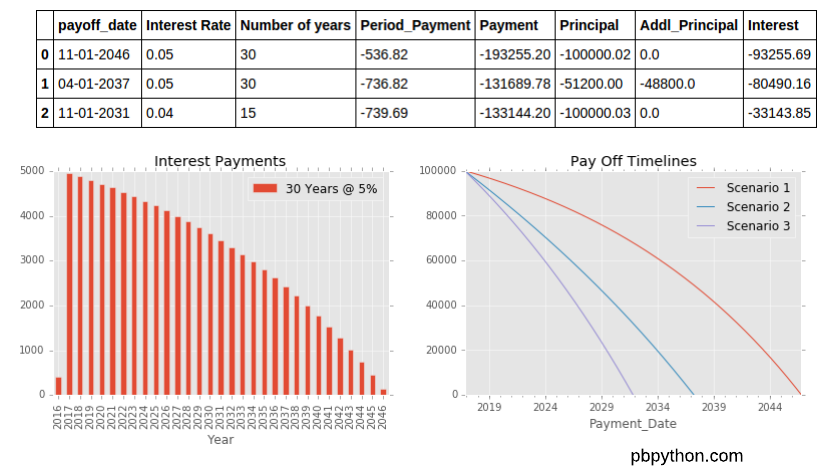
This article from Practical Business Python demonstrates a similar principle. While the model itself is for loan amortization, the key lesson is in the "Time to Analyze" section, where the author wraps the model logic into a function to run multiple scenarios.
Read the section "Time to Analyze". Focus on how the author creates an amortization_table function. Notice how this function takes key drivers (like interest_rate, years, principal) as arguments. We will do the same, but our argument will be a dictionary containing all our assumptions. Also, observe how the author then runs multiple scenarios and combines the results using pd.concat.
Here is our refactored code. The logic is identical to our previous lessons, but it's now neatly contained within a function.
import pandas as pd
import numpy as np
import matplotlib.pyplot as plt

def run_financial_model(assumptions):
    """
    Runs a 3-statement financial model for a given set of assumptions.

    Args:
        assumptions (dict): A dictionary containing all the necessary model drivers.

    Returns:
        tuple: A tuple containing the projected Income Statement, Balance Sheet, and Cash Flow Statement as pandas DataFrames.
    """
    years = ['2021A', '2022A', '2023A', '2024F', '2025F', '2026F']
    forecast_years = ['2024F', '2025F', '2026F']


    # --- Income Statement ---
    projected_is = pd.DataFrame(index=['Sales'], columns=years)


    # Historical Sales
    projected_is.loc['Sales', ['2021A', '2022A', '2023A']] = [150.0, 170.0, 195.0]


    # Forecast Sales
    for i in range(3, len(years)):
        projected_is.loc['Sales', years[i]] = projected_is.loc['Sales', years[i-1]] * (1 + assumptions['sales_growth'])

    projected_is.loc['COGS'] = projected_is.loc['Sales'] * -assumptions['cogs_margin']
    projected_is.loc['Gross Profit'] = projected_is.loc['Sales'] + projected_is.loc['COGS']
    projected_is.loc['SG&A'] = projected_is.loc['Sales'] * -assumptions['sga_margin']
    projected_is.loc['Depreciation'] = projected_is.loc['Sales'] * -assumptions['depr_margin']
    projected_is.loc['EBIT'] = projected_is.loc['Gross Profit'] + projected_is.loc['SG&A'] + projected_is.loc['Depreciation']
    projected_is.loc['Interest Expense'] = 0 # Simplified
    projected_is.loc['EBT'] = projected_is.loc['EBIT'] + projected_is.loc['Interest Expense']
    projected_is.loc['Tax'] = -projected_is.loc['EBT'].apply(lambda x: x * assumptions['tax_rate'] if x > 0 else 0)
    projected_is.loc['Net Income'] = projected_is.loc['EBT'] + projected_is.loc['Tax']


    # --- Balance Sheet ---
    projected_bs = pd.DataFrame(columns=years)


    # Seed historical values
    projected_bs.loc['Cash', '2023A'] = 30.0
    projected_bs.loc['Accounts Receivable', '2023A'] = 25.0
    projected_bs.loc['Inventory', '2023A'] = 20.0
    projected_bs.loc['PP&E', '2023A'] = 100.0
    projected_bs.loc['Accounts Payable', '2023A'] = 15.0
    projected_bs.loc['Retained Earnings', '2023A'] = 80.0


    # Project BS items linked to IS
    projected_bs.loc['Accounts Receivable'] = (assumptions['ar_days']/365) * projected_is.loc['Sales']
    projected_bs.loc['Inventory'] = (assumptions['inv_days']/365) * -projected_is.loc['COGS']
    projected_bs.loc['Accounts Payable'] = (assumptions['ap_days']/365) * -projected_is.loc['COGS']

    capex = projected_is.loc['Sales'] * assumptions['capex_margin']
    depreciation_val = -projected_is.loc['Depreciation']
    dividends = -projected_is.loc['Net Income'] * assumptions['dividend_payout']

    for year_idx in range(3, len(years)):
        prev_year = years[year_idx - 1]
        curr_year = years[year_idx]
        projected_bs.loc['PP&E', curr_year] = projected_bs.loc['PP&E', prev_year] + capex[curr_year] - depreciation_val[curr_year]
        projected_bs.loc['Retained Earnings', curr_year] = projected_bs.loc['Retained Earnings', prev_year] + projected_is.loc['Net Income', curr_year] + dividends[curr_year]


    # --- Cash Flow Statement ---
    projected_cfs = pd.DataFrame(columns=forecast_years)
    bs_changes = projected_bs.diff(axis=1)
    cfo = projected_is.loc['Net Income', forecast_years] + depreciation_val[forecast_years] - bs_changes.loc['Accounts Receivable', forecast_years] - bs_changes.loc['Inventory', forecast_years] + bs_changes.loc['Accounts Payable', forecast_years]
    projected_cfs.loc['CFO'] = cfo
    projected_cfs.loc['CFI'] = -capex[forecast_years]
    projected_cfs.loc['CFF'] = dividends[forecast_years]
    projected_cfs.loc['Net Change in Cash'] = projected_cfs.sum()


    # --- Link CFS to BS ---
    for year_idx in range(3, len(years)):
        prev_year = years[year_idx - 1]
        curr_year = years[year_idx]
        projected_bs.loc['Cash', curr_year] = projected_bs.loc['Cash', prev_year] + projected_cfs.loc['Net Change in Cash', curr_year]


    # --- Validation ---
    asset_items = ['Cash', 'Accounts Receivable', 'Inventory', 'PP&E']
    liab_equity_items = ['Accounts Payable', 'Retained Earnings']
    projected_bs.loc['Total Assets'] = projected_bs.loc[asset_items].sum()
    projected_bs.loc['Total Liabilities & Equity'] = projected_bs.loc[liab_equity_items].sum()
    projected_bs.loc['Balance Check'] = projected_bs.loc['Total Assets'] - projected_bs.loc['Total Liabilities & Equity']

    assert np.allclose(projected_bs.loc['Balance Check', forecast_years].values, 0), "Model does not balance!"

    return projected_is, projected_bs, projected_cfs
Step 3: Iterate, Analyze, and Visualize
With our function and scenarios defined, the final step is to loop through them, run the model for each, and then aggregate and visualize the results. We will store the key outputs in a dictionary and then use pandas.concat to create a combined DataFrame for easy comparison.
# Create a dictionary to hold the results from each scenario
results = {}


# Loop through each scenario, run the model, and store the income statement
for scenario_name, assumption_set in scenarios.items():
    is_proj, _, _ = run_financial_model(assumption_set)
    results[scenario_name] = is_proj.loc['Net Income', forecast_years]


# Combine the results into a single DataFrame
results_df = pd.DataFrame(results)

print("--- Net Income Projections by Scenario ---")
print(results_df.round(1))


# --- Visualize the results ---
results_df.plot(kind='bar', figsize=(10, 6))
plt.title('Projected Net Income by Scenario')
plt.ylabel('Net Income ($)')
plt.xlabel('Forecast Year')
plt.xticks(rotation=0)
plt.grid(axis='y', linestyle='--', alpha=0.7)
plt.legend(title='Scenario')
plt.tight_layout()
plt.show()
When you execute this code, you'll get a clear table and a bar chart comparing the Net Income for the base, bull, and bear cases across the forecast years. You can immediately see the financial impact of the different strategic assumptions.
This programmatic approach is far more powerful than a manual one. If you wanted to add a fourth "hyper-growth" scenario or test the impact of changing tax rates, you would only need to add a new dictionary to scenarios and re-run the script. The model logic itself remains untouched, minimizing the risk of errors.
Conclusion
In this lesson, you have taken a major step from being a model builder to a model user. You've learned how to leverage your validated financial model to perform scenario analysis, a cornerstone of strategic financial planning.
Key Takeaways:
- Scenario analysis is a technique for exploring different future outcomes by creating discrete cases (e.g., base, bull, bear) with varying sets of assumptions.
- The best practice for implementing this in Python is to separate assumptions from logic. We used dictionaries to define our scenarios.
- Encapsulating model logic into a function is a powerful technique that makes your model reusable, testable, and scalable for running multiple scenarios.
- Using
pandasto aggregate results andmatplotlibto visualize them allows for clear and impactful analysis of the different scenarios.
This lesson concludes our module on the foundations of financial modeling. You have built a robust, three-statement model from scratch, learned to validate it, and used it for strategic scenario analysis.
In our next module, we will dive into Company Valuation with DCF Analysis. We will take the projected financials you've just generated and use them to calculate one of the most important metrics in finance: a company's intrinsic value. The scenario analysis framework you built today will be invaluable, as we will be able to see not just how profits change, but how the entire valuation of the business shifts under different strategic assumptions.