Hello! Welcome back to our course on preparing for senior backend engineer interviews.
In our last lesson, we focused on schema design, comparing normalization for write-heavy workloads and denormalization for read-heavy ones. We briefly touched upon indexing as a primary tool for optimizing read performance. Today, we're going to do a deep dive into that exact topic.
The learning outcome for this lesson is to explain database indexing strategies and their performance implications. This is a fundamental concept in system design, and your ability to discuss the trade-offs between different indexing mechanisms, particularly B-Trees and LSM-Trees, is a strong signal of seniority. We'll move beyond just knowing what an index is and focus on the underlying data structures to understand why they perform differently.
1. The Core Problem: Why Do We Need Indexes?
Before we dive into different strategies, let's solidify our understanding of the problem indexes solve. Without an index, when you query for a specific row, the database has no choice but to perform a full table scan—reading every single row until it finds a match. For a table with millions or billions of rows, this is unacceptably slow.
DB Indexing in System Design Interviews - B-tree, Geospatial, Inverted Index, and more!
To start, let's watch a short, clear explanation of this problem from the 'Hello Interview' channel. It quantifies the performance difference and introduces the basic concept of an index as a lookup structure.
Please watch from 00:30 to 02:10. Focus on the comparison between a sequential scan and an index-based lookup, and how the index acts as a map to the data's location on disk.
As the video explains, an index is essentially an auxiliary data structure that provides a shortcut to the data, dramatically reducing the number of disk reads required. The choice of which data structure to use for this index has profound performance implications. Let's explore the two most important ones.
2. The Default Workhorse: B-Tree Indexes
For decades, the B-Tree has been the standard, default data structure for indexing in most relational databases like PostgreSQL, MySQL, and Oracle. As a backend engineer, you've used B-Tree indexes countless times, even if you weren't thinking about the underlying mechanics.
DB Indexing in System Design Interviews - B-tree, Geospatial, Inverted Index, and more!
Let's continue with the same video to understand how a B-Tree works at a high level.
Watch the segment from 02:10 to 04:05. Pay attention to how the tree structure allows for efficient traversal for both exact matches (= 51) and range queries (> 51).
A B-Tree (Balanced Tree) is a self-balancing tree data structure that keeps data sorted and allows searches, sequential access, insertions, and deletions in logarithmic time. Here are its key characteristics:
- Structure: It's a tree of "pages" or "blocks" on disk. The root node points to child nodes, which in turn point to other nodes, until you reach the leaf nodes that contain pointers to the actual table rows.
- Performance:
- Reads are fast and predictable. Finding any piece of data takes a number of disk seeks proportional to the height of the tree, which is very shallow even for massive tables (e.g., a 4-level tree can index trillions of rows). This makes B-Trees excellent for read-heavy and mixed workloads.
- Writes are slower. When you insert or update a value, the database must find the correct page on disk and modify it in place. If the page is full, it must be split, which can trigger a cascade of updates up the tree. This "read-modify-write" pattern makes writes more expensive than reads.
A Note on B+ Trees
In practice, most databases use a variation called a B+ Tree. The main difference is that in a B+ Tree, all the actual data pointers are stored only in the leaf nodes, and these leaf nodes are linked together in a doubly-linked list.
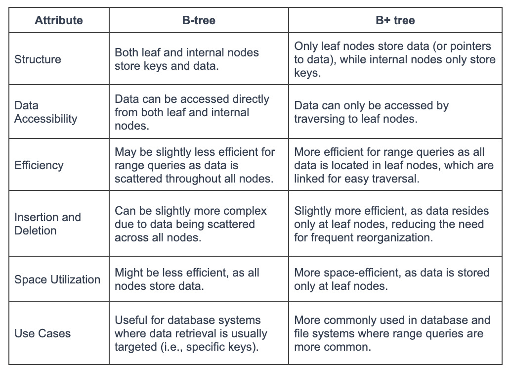
This linked-list structure makes range queries (e.g., WHERE age BETWEEN 30 AND 40) extremely efficient, as the database can find the start of the range and then just scan across the leaf nodes.
3. The Write-Optimized Alternative: LSM-Trees
In our last lesson, we mentioned that some databases are specifically designed for write-heavy workloads. The magic behind their performance is often a different indexing structure: the Log-Structured Merge-Tree (LSM-Tree). Databases like Cassandra, ScyllaDB, and RocksDB use this approach.
An LSM-Tree turns the B-Tree's write model on its head. Instead of modifying pages on disk, it treats the database file like a log and only appends data.
This concept can be broken down into a few key components:
- Memtable: A sorted, in-memory data structure (like a balanced binary search tree). All new writes go directly here, which is extremely fast.
- Write-Ahead Log (WAL): A log file on disk where every write is also appended. This provides durability in case the server crashes before the memtable is saved.
- SSTables (Sorted String Tables): When the memtable reaches a certain size, it's flushed to disk as an immutable, sorted file called an SSTable.
- Compaction: A background process periodically merges these SSTables, cleaning up old or deleted values and combining smaller segments into larger ones.
LSM Tree + SSTable Database Indexes | Systems Design Interview: 0 to 1 with Google Software Engineer
The video 'LSM Tree + SSTable Database Indexes' by Jordan has no life provides a fantastic, detailed walkthrough of this process. We'll watch it in a few parts.
First, watch from 00:24 to 04:41. This section covers the core concepts: the in-memory tree (memtable), the need for a WAL for durability, and the process of flushing the memtable to an on-disk SSTable.
Now that we understand how data gets written, how do we read it back? A read has to check for the key in multiple places, in order:
- Check the in-memory memtable.
- If not found, check the most recent SSTable on disk.
- If not found, check the next SSTable, and so on.
LSM Tree + SSTable Database Indexes | Systems Design Interview: 0 to 1 with Google Software Engineer
Let's continue with the same video to see how reads work and how LSM-Trees are optimized.
Now watch from 04:41 to 12:06. This part explains the read path, how deletions are handled with 'tombstones', and crucial optimizations like sparse indexes and Bloom filters (which quickly tell you if a key is not in an SSTable, avoiding a costly disk scan). It also covers the compaction process.
4. B-Tree vs. LSM-Tree: The Interview Trade-off Framework
This is the most critical part for your interviews. You need to be able to articulate the trade-offs between these two strategies clearly.
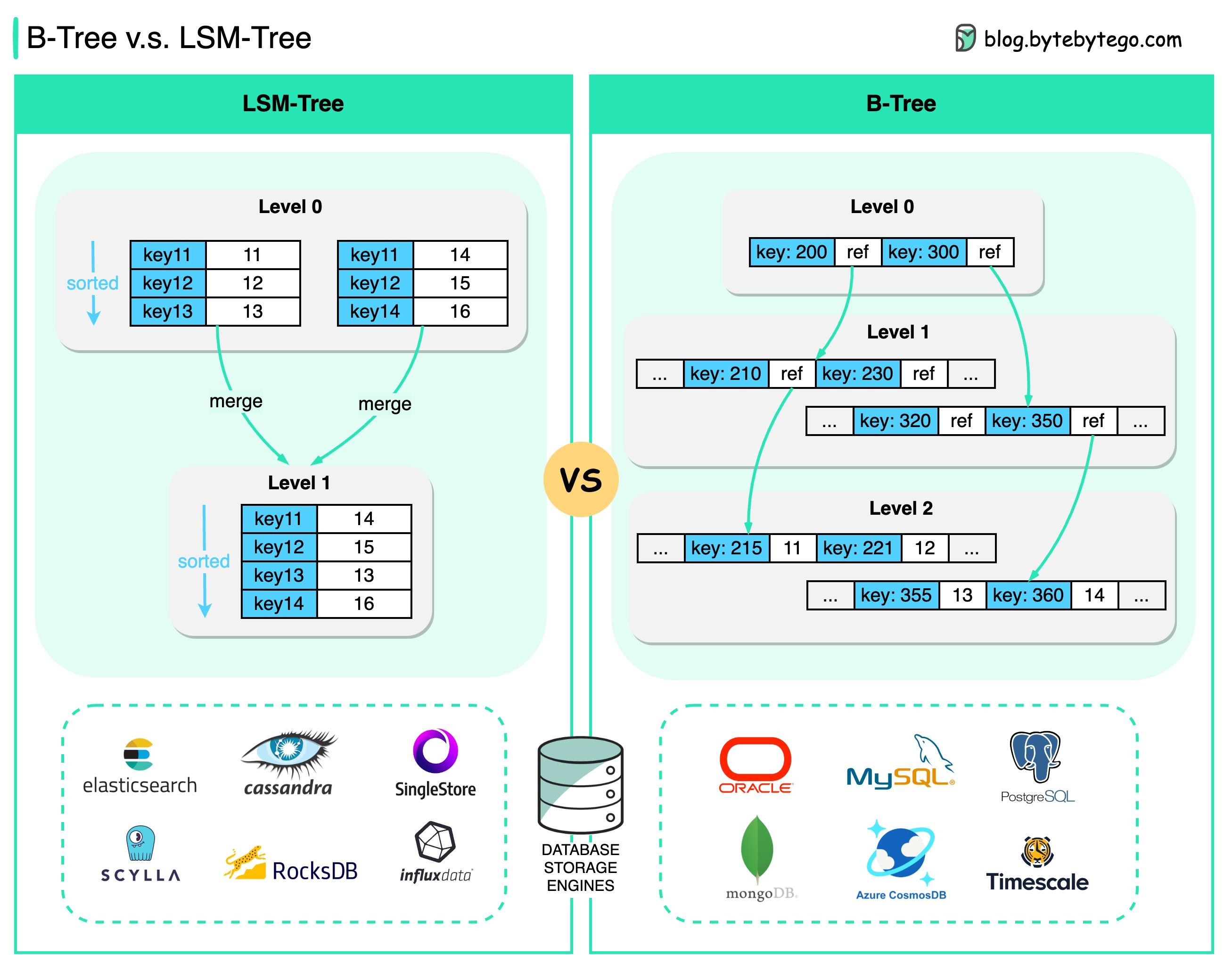
Here's a summary table you can use as a mental model:
| Characteristic | B-Tree (e.g., PostgreSQL, MySQL) | LSM-Tree (e.g., Cassandra, RocksDB) |
|---|---|---|
| Write Performance | Slower. Writes are "in-place" and can cause page splits and locking. High write load can lead to contention. | Faster. Writes are sequential appends to an in-memory table and a WAL. Very high write throughput. |
| Read Performance | Faster and more predictable. Each key exists in exactly one place in the index. Lookups require a single tree traversal. | Potentially slower. A key's latest value might be in the memtable or any of several SSTables, requiring multiple lookups. Can suffer from high read latency if not tuned. |
| Compaction | Not applicable in the same way. | Essential but complex. Background compaction is required to merge SSTables and reclaim space. This can consume significant I/O and CPU. |
| Space Usage | More efficient. No data duplication in the index itself. | Less efficient. Old/updated data exists in old SSTables until compaction runs, leading to space amplification. |
| Best For... | General purpose, read-heavy, or mixed OLTP workloads where transactions and strong consistency are key. | Write-heavy workloads like logging, time-series data, event sourcing, or analytics ingestion. |
LSM Tree + SSTable Database Indexes | Systems Design Interview: 0 to 1 with Google Software Engineer
To reinforce this comparison, let's watch the concluding summary from the 'LSM Tree' video.
Watch from 12:06 to 15:14. The speaker provides a final comparison of Hash Indexes, B-Trees, and LSM-Trees, summarizing their pros and cons for different use cases.
5. Specialized Indexing Strategies
For a senior role, it's also important to know that B-Trees and LSM-Trees aren't the only options. Certain query types require specialized indexes. Mentioning these demonstrates breadth of knowledge.
Full-Text Search: Inverted Index
A B-Tree is great for prefix searches (name LIKE 'John%') but terrible for suffix or contains searches (name LIKE '%Smith'). For this, you need an inverted index.
An inverted index maps terms (words) to the documents that contain them. Search engines like Elasticsearch and Solr are built on this concept.
Geospatial Data: R-Trees and Geohashes
A B-Tree indexes one-dimensional data. Trying to query two-dimensional data (latitude and longitude) for "nearby" locations is inefficient. Specialized geospatial indexes solve this.
- R-Trees: A tree structure that groups nearby objects into "minimum bounding rectangles." Used by PostGIS.
- Geohashing: A technique that encodes a 2D location into a short, one-dimensional string, where similar prefixes correspond to nearby locations. You can then build a standard B-Tree on these hash strings.
DB Indexing in System Design Interviews - B-tree, Geospatial, Inverted Index, and more!
The 'Hello Interview' video provides a great, high-level overview of these specialized indexes, which is exactly the level of detail you need for most system design interviews.
Watch from 05:05 to 12:39. This covers geospatial indexes (geohashing, quad-trees, R-trees) and inverted indexes for full-text search.
Conclusion
Understanding indexing is not just about knowing when to add CREATE INDEX. For a senior engineer, it's about understanding the fundamental trade-offs between the underlying data structures and choosing a database or strategy that matches your workload's access patterns.
Key Takeaways:
- B-Trees are the default index for most relational databases. They offer excellent, predictable read performance but have slower writes. They are ideal for mixed OLTP workloads.
- LSM-Trees are optimized for very high write throughput by turning random writes into sequential appends. Read performance can be less predictable. They are ideal for write-heavy systems like logging and analytics platforms.
- The choice between B-Tree and LSM-Tree based systems is a core architectural decision that depends on whether your workload is read-heavy or write-heavy.
- Specialized queries require specialized indexes: inverted indexes for full-text search and geospatial indexes for location-based queries.
In our next lesson, we'll move from single-node performance to multi-node scalability and reliability. We will describe database replication patterns (master-slave, master-master) and their trade-offs, a critical topic for building resilient and scalable systems.