Designing Time-Series Metrics Systems

1. Defining the System: Requirements and Scope

As always, we begin by clarifying the problem. A metrics system can be vast, so we need to define a clear set of functional and non-functional requirements to guide our design.

Let's start by outlining what our system must do. A good set of requirements forms the foundation of a strong design.

Based on that reading and common expectations for this problem, here is our refined scope:

Functional Requirements:

1. Collect Metrics: The system must gather metrics from millions of sources (servers, applications, devices). Metrics include CPU utilization, memory usage, request latency, error counts, etc.
2. Store Metrics: Store the collected time-series data efficiently.
3. Aggregate & Downsample: Provide aggregated views of data over different time windows (e.g., average CPU over the last hour, day, or month).
4. Query & Visualize: Expose an API for querying the data, which will be used by dashboards (like Grafana) to display graphs and charts.
5. Alerting: Allow users to define rules (e.g., "alert if CPU > 90% for 5 minutes") and trigger notifications.

Non-Functional Requirements:

1. High Write Throughput: The system must handle millions of metric data points per second. This is a write-heavy system.
2. Low Query Latency: Queries for recent data (e.g., last hour) for dashboards should be very fast (sub-second).
3. Scalability: The architecture must scale horizontally to accommodate growth in the number of metrics and sources.
4. Reliability & Durability: The system should not lose metric data, and the alerting component must be highly reliable.
5. Cost-Effectiveness: Manage storage costs through data retention policies and compression.

The fundamental data point we are dealing with has a specific structure, which is crucial for the entire design.

A metric data point is typically composed of:

• Metric Name: e.g., cpu.utilization
• Timestamp: The time the measurement was taken (e.g., a Unix epoch).
• Value: The measured value (e.g., 0.75).
• Tags/Labels: Key-value pairs that add context, like host=server-123, region=us-east-1. These are critical for filtering and aggregation.

2. High-Level Architecture

Now, let's sketch out the main components of our system. The architecture can be broken down into a pipeline: collection, ingestion, storage, processing, and consumption (querying, alerting).

The initial design introduces several key ideas. Let's formalize the data collection models and then address the obvious scalability bottleneck.

Data Collection: Push vs. Pull

There are two primary models for getting data from the sources to our collection service:

1. Push Model: An agent running on each source actively sends metrics to a central endpoint. This is simpler for dynamic environments (e.g., serverless functions, short-lived jobs) as the source doesn't need to be discoverable.
2. Pull Model: A central collector periodically scrapes a /metrics endpoint on each source. This gives the monitoring system more control and doubles as a health check (if a scrape fails, the source is likely down).

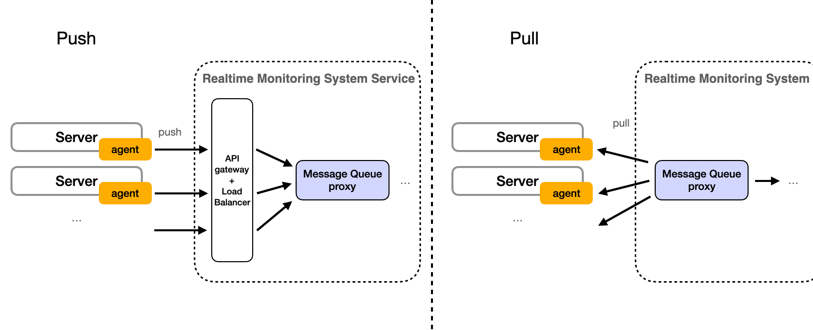
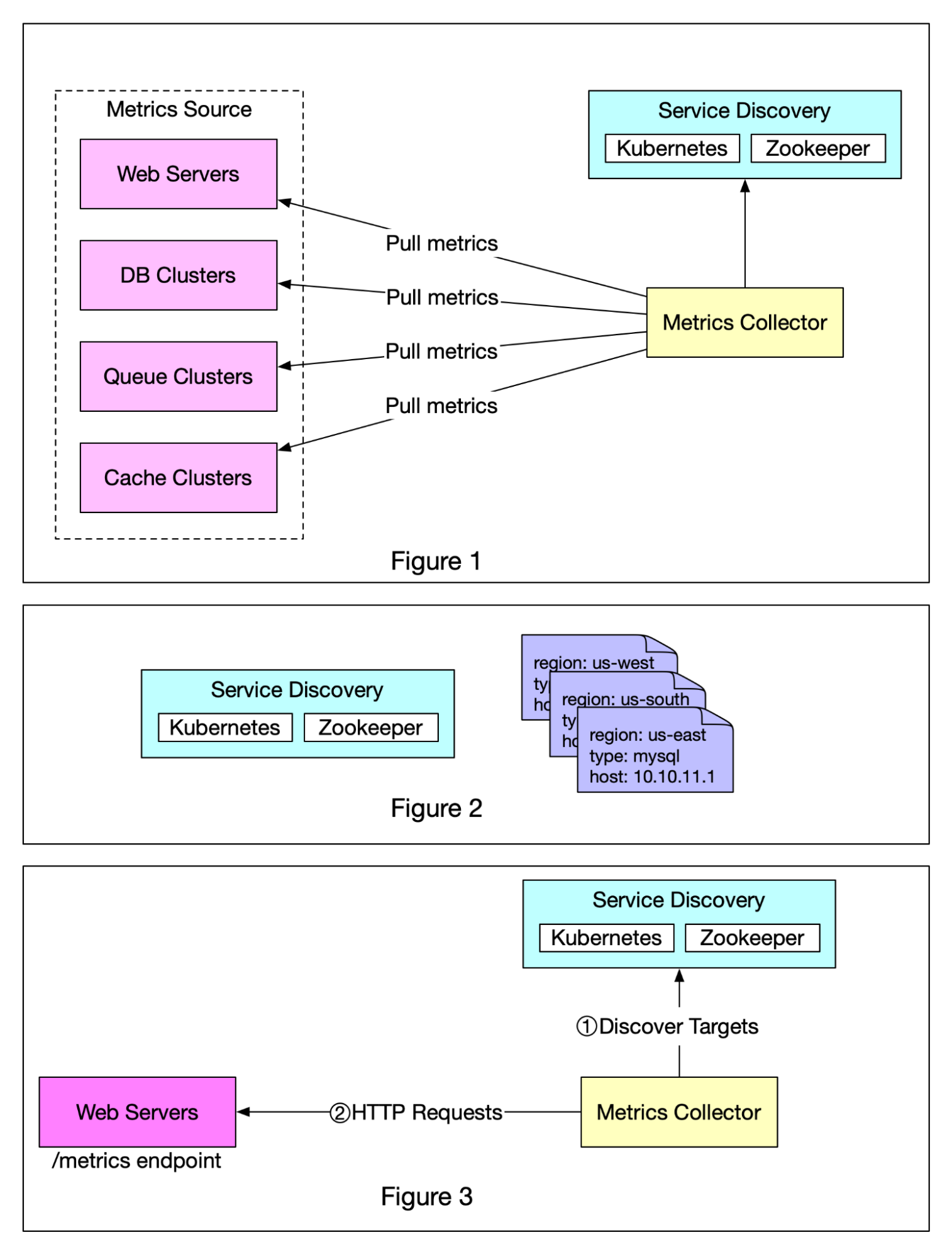
For a large, heterogeneous environment, a hybrid approach supporting both models is often best.

Scaling the Ingestion Pipeline

The simple design from the video (Agent -> Collector -> DB) has a major bottleneck: the collector service and the database will be overwhelmed by the high write volume. Your experience with backend systems should immediately flag this as a point of failure.

The solution is to decouple the write path using a message queue.

Our scaled-up high-level architecture now looks like this:

1. Metric Sources (with Agents) send metrics.
2. A Load Balancer distributes the incoming traffic across a fleet of stateless Collector Services.
3. The collectors publish the metrics to a Message Queue (like Apache Kafka). This queue acts as a durable buffer, absorbing write spikes.
4. A set of Consumer/Processor Services read from the queue.
5. These services write the data to a specialized Time-Series Database (TSDB).
6. A Query Service provides an API for reading data from the TSDB.
7. Dashboards and an Alerting System use the Query Service.

3. Deep Dive: The Time-Series Database (TSDB)

The choice of database is the most critical decision in this design. Why can't we just use a standard SQL database like PostgreSQL, or a general-purpose NoSQL store like Cassandra?

The answer lies in the unique characteristics of time-series data: an extremely high volume of writes, append-only operations, and queries that are almost always filtered and aggregated by time. This workload requires a purpose-built solution.

This next video is a masterclass on the internal workings of TSDBs. Understanding these principles is what interviewers at top companies look for in a senior candidate.

Part A: Why Not Relational Databases?

First, let's understand the problem we're solving.

Part B: Optimizing for High-Throughput Writes

To handle millions of writes per second, TSDBs use a storage engine structure that favors sequential writes. The Log-Structured Merge (LSM) Tree is a perfect example.

Part C: Optimizing for Storage and Queries

TSDBs employ clever tricks to reduce storage footprint and speed up queries.

Part D: The Achilles' Heel - Cardinality

The biggest performance challenge for TSDBs is high cardinality. Cardinality refers to the number of unique time series, which is determined by the unique combinations of a metric name and its tags.

4. Aggregation and Data Lifecycle

As we saw, downsampling is a key feature of TSDBs. In our system design, we need to formalize this into a concrete data lifecycle and retention policy. This is essential for managing storage costs and maintaining query performance.

We will define a tiered retention strategy:

• Hot Tier: Raw, high-resolution data (e.g., 10-second granularity) is kept for a short period (e.g., 7 days) in the fastest storage for real-time dashboards and immediate debugging.
• Warm Tier: Data is downsampled to a lower resolution (e.g., 1-minute granularity) and kept for a medium term (e.g., 30-90 days). This is used for trend analysis over recent weeks.
• Cold Tier: Data is further downsampled (e.g., 1-hour granularity) and kept for a long term (e.g., 1-2 years) for historical reporting. For compliance, raw data might be moved from the ingestion pipeline to cheap, long-term object storage like Amazon S3.

The video below discusses this concept of having a real-time path for dashboards and a separate path for raw data archiving.

Conclusion

In this lesson, we designed a scalable and robust time-series metrics collection and aggregation system. We moved from basic requirements to a sophisticated, decoupled architecture and dove deep into the specialized technologies that make it possible.

Key Takeaways:

• Decouple for Scale: Use a message queue like Kafka to buffer the massive write load, allowing the collection and storage tiers to scale independently.
• Use the Right Tool: Time-series data has a unique workload. A purpose-built Time-Series Database (TSDB) is essential for performance.
• Understand TSDB Internals: For a senior-level discussion, you should be able to explain why TSDBs are fast, referencing concepts like LSM trees for writes and delta encoding for compression.
• Beware High Cardinality: The number of unique time series is a critical performance factor. Avoid using high-cardinality identifiers (like user_id) as tags.
• Implement a Data Lifecycle: Use downsampling and tiered storage (hot, warm, cold) to balance query performance, data granularity, and storage cost.

Next Lesson Preview:

We've now completed several complex system design problems. Your goal, however, isn't just to be a great designer but to prove it in an interview. The other half of that challenge is the behavioral interview. In our next lesson, we will shift gears and begin our module on Behavioral Interview Fundamentals. We'll start by learning to describe the purpose and evaluation criteria of behavioral interviews and introduce the famous STAR method for structuring your answers.