Solving Electrostatic Boundary-Value Problems with Poisson's and Laplace's Equations

1. The Differential Equations of the Electrostatic Potential

Our entire theory of electrostatics rests on two fundamental differential laws you've seen before:

1. Gauss's Law (differential form): $\nabla \cdot \mathbf{E}=\frac{\rho }{{ϵ}_0}$
2. The Conservative Nature of $\mathbf{E}$: $\nabla \times \mathbf{E}=0$, which implies $\mathbf{E}=-\nabla V$

By combining these two laws, we can derive a single master equation for the scalar potential $V$. This is a cornerstone of potential theory.

As you saw in the video, substituting $\mathbf{E}=-\nabla V$ into $\nabla \cdot \mathbf{E}=\rho /{ϵ}_0$ gives:
$\nabla \cdot (-\nabla V)=\frac{\rho }{{ϵ}_0}$
This leads to Poisson's equation:
${\nabla }^{2}V=-\frac{\rho }{{ϵ}_0}$
Here, ${\nabla }^2$ (del-squared) is the Laplacian operator. In Cartesian coordinates, it is ${\nabla }^2=\frac{{\partial }^2}{\partial x^2}+\frac{{\partial }^2}{\partial y^2}+\frac{{\partial }^2}{\partial z^2}$.

In a region of space where there are no free charges ($\rho =0$), Poisson's equation simplifies to Laplace's equation:
${\nabla }^{2}V=0$
Laplace's equation is particularly important because it governs the potential in the vast empty spaces between and around conductors, which are often held at fixed potentials. This setup defines what we call a boundary-value problem: we know the value of the potential $V$ on the surfaces of a region (the "boundary conditions") and we want to find $V$ everywhere inside that region.

2. Uniqueness and Properties of Solutions

Before we start solving these equations, a crucial theoretical question arises: if we find a solution that satisfies the boundary conditions, is it the only possible solution? The answer is yes, and this is guaranteed by the Uniqueness Theorem.

This theorem is what makes boundary-value problems so powerful. It tells us that if we can find a solution by any method—no matter how strange—and it fits the boundary conditions, it is the correct and only solution.

Another key property of solutions to Laplace's equation is that they have no local maxima or minima. The extreme values of the potential must occur on the boundaries of the region.

3. Solving 1D Boundary-Value Problems

The simplest boundary-value problems are those where symmetry dictates that the potential $V$ only varies with one coordinate (e.g., $V(x)$, $V(\rho )$, or $V(r)$). In these cases, the partial differential equation (PDE) becomes a simple ordinary differential equation (ODE) that you can solve by direct integration.

The general procedure is:

1. Solve the ODE to get a general solution with integration constants (e.g., A and B).
2. Apply the given boundary conditions to determine the values of these constants.
3. Use $\mathbf{E}=-\nabla V$ to find the electric field.

Let's look at some examples from the Sadiku textbook.

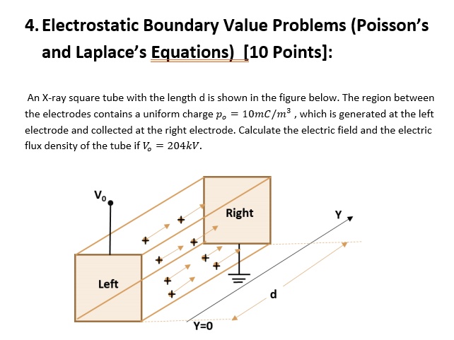
Example 1: Cartesian Coordinates (An Engineering Application)

Consider the model of an electrohydrodynamic (EHD) pump. This is a real-world device where an electric field is used to pump fluids.

Example 2: Spherical Coordinates

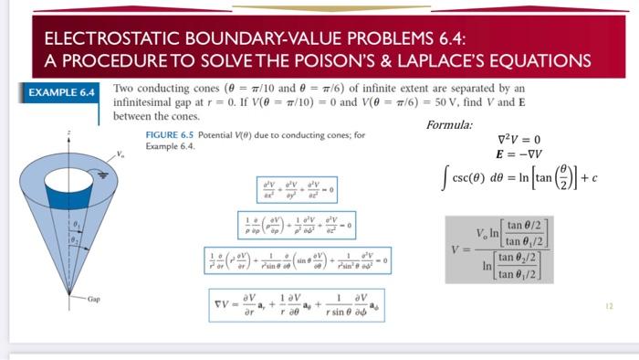
Now consider two conducting cones held at different potentials. The symmetry suggests that the potential $V$ depends only on the polar angle $\theta$.

4. Solving 2D Problems: The Method of Separation of Variables

When the potential depends on more than one variable, we can't just integrate directly. The most important analytical technique for solving Laplace's equation is the method of separation of variables. The core idea is to assume the solution is a product of functions, each depending on only one variable: for instance, $V(x,y)=X(x)Y(y)$. This assumption converts the single PDE into a set of simpler ODEs.

Let's see this in action with a classic example: a rectangular trough with three grounded sides and one side held at a constant potential $V_0$.

This method is extremely general. The same process is used in cylindrical or spherical coordinates, though the resulting ODEs (like Bessel's equation or Legendre's equation) and their solutions (special functions) are more complex. The NPTEL video LINK you looked at earlier shows the derivation for spherical coordinates, leading to Legendre Polynomials, which are essential in many areas of advanced physics.

Conclusion

Today, we've transitioned from solving electrostatic problems with integration to solving them with partial differential equations. This is a significant step up in sophistication and power.

Key Takeaways:

• Combining Gauss's Law with $\mathbf{E}=-\nabla V$ gives Poisson's equation (${\nabla }^{2}V=-\rho /{ϵ}_0$) and Laplace's equation (${\nabla }^{2}V=0$).
• These equations, along with specified boundary conditions, form a boundary-value problem.
• The Uniqueness Theorem guarantees that if we find one solution to a boundary-value problem, it is the only one.
• Solutions to Laplace's equation are "smooth" and have their maximum and minimum values on the boundary, not in the interior.
• 1D problems can be solved by direct integration of the corresponding ODE.
• Higher-dimensional problems are typically solved with the method of separation of variables, which transforms the PDE into a set of ODEs and often results in a Fourier series solution.

Preview of the Next Lesson:
In our next lesson, we will focus on the behavior of conductors in electrostatic equilibrium. We will see that the entire volume of a conductor is an equipotential region, which provides a powerful boundary condition for solving Laplace's equation. This will also allow us to formally define capacitance and justify an elegant problem-solving shortcut called the method of images, whose validity rests on the uniqueness theorem you learned today.