Deriving the Equation of Motion for SHM

1. The Equation of Motion for SHM

Let's consider the archetypal example of SHM: a mass $m$ attached to a horizontal spring with spring constant $k$, sliding on a frictionless surface.

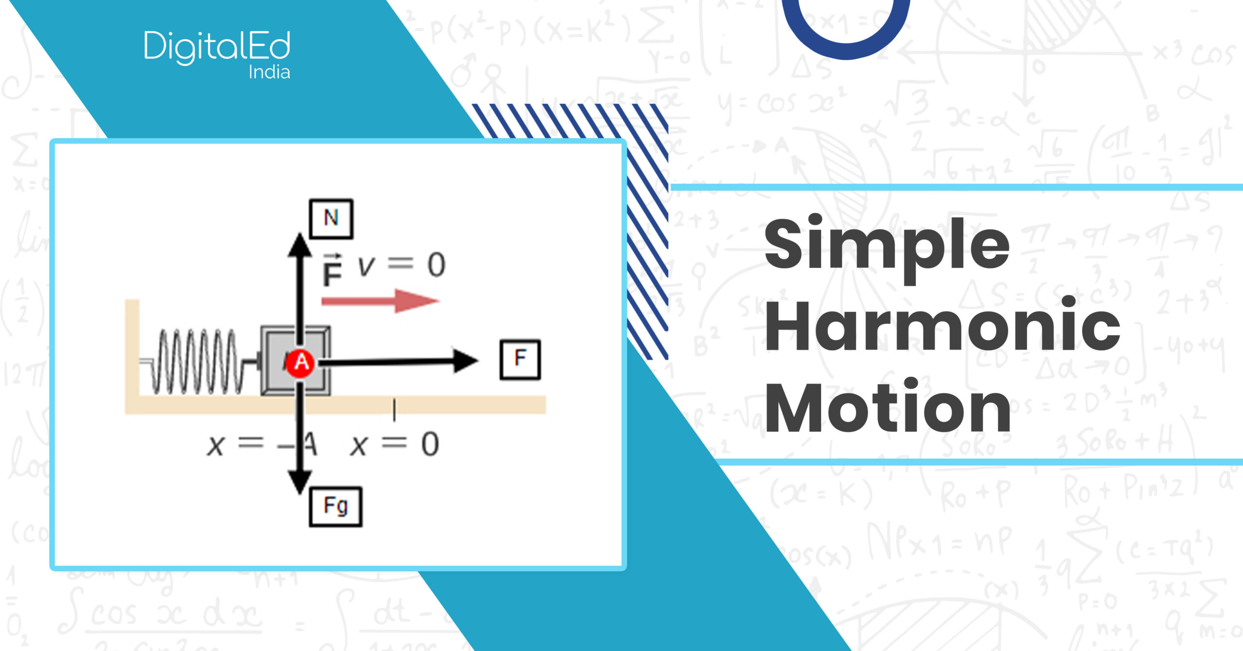
We can derive the equation of motion by following these steps:

1. Identify the Force: According to Hooke's Law, an ideal spring exerts a restoring force that is linearly proportional to the displacement $x$ from its equilibrium position. The negative sign indicates the force is always directed opposite to the displacement.

   $$F_{spring}=-kx$$

2. Apply Newton's Second Law: The net force on the mass causes it to accelerate.

   $$F_{net}=ma=m\frac{d^{2}x}{d{t}^2}$$

3. Combine the Laws: By equating the two expressions for the force, we get the equation of motion for the mass-spring system.

   $$m\frac{d^{2}x}{d{t}^2}=-kx$$

Rearranging this equation gives us the standard form of the Simple Harmonic Oscillator (SHO) equation:

This is a second-order, linear, homogeneous ordinary differential equation with constant coefficients. Its properties are central to all of physics.

We define the natural angular frequency ${\omega }_0$ as:

This intrinsic frequency depends only on the physical properties of the system (mass and spring stiffness). The SHO equation can now be written more compactly as:

where $\ddot{x}$ is shorthand for $\frac{d^{2}x}{d{t}^2}$.

For a clear walkthrough of this derivation, watch the beginning of the following video.

This same mathematical form appears in many other physical systems. For example, a simple pendulum of length $l$ oscillating at small angles $\theta$ is described by $\ddot{\theta }+(g/l)\theta \approx 0$. This shows the universality of the SHO equation.

2. Solving the SHO Equation

Now that we have the equation, how do we find the function $x(t)$ that describes the position of the mass over time? Since this is a differential equation, its solution isn't just a number, but a function. We will explore two key methods.

Method 1: The "Physics Guess" - Sinusoidal Solutions

Our physical intuition tells us that the mass will oscillate back and forth. The simplest mathematical functions that describe oscillation are sines and cosines. Let's make an educated guess (an ansatz) that the solution is a combination of these:

where $C$ and $D$ are constants. To verify this, we take two derivatives:

So, we have $\ddot{x}(t)=-{\omega }_0^{2}x(t)$, which is exactly our SHO equation $\ddot{x}+{\omega }_0^{2}x=0$. Our guess is correct!

The constants $C$ and $D$ are determined by the initial conditions of the motion—the position $x_0$ and velocity $v_0$ at $t=0$.

• At $t=0$, $x(0)=C\cos (0)+D\sin (0)=C$. So, $C=x_0$.
• At $t=0$, $\dot{x}(0)=-C{\omega }_0\sin (0)+D{\omega }_0\cos (0)=D{\omega }_0$. So, $D=v_0/{\omega }_0$.

Therefore, the specific solution for a given set of initial conditions is:

The following reading provides a detailed, step-by-step derivation of this general solution and how to determine the constants from initial conditions.

Method 2: The Systematic Approach - Complex Exponentials

While guessing works well here, a more powerful and systematic method for linear ODEs uses complex numbers. This approach is fundamental in advanced physics and engineering.

We guess a solution of the form $x(t)=e^{\lambda t}$. The beauty of the exponential function is that its derivative is proportional to itself. Substituting this into $\ddot{x}+{\omega }_0^{2}x=0$ gives:

Since $e^{\lambda t}$ is never zero, we can divide it out, leaving the characteristic equation:

This gives us two complex solutions: $e^{i{\omega }_{0}t}$ and $e^{-i{\omega }_{0}t}$.

Because the SHO equation is linear, any linear combination of solutions is also a solution (this is the principle of superposition). So, the general complex solution is:

However, the position $x$ must be a real number. For $x(t)$ to be real, it must equal its own complex conjugate, $x(t)=x^{\ast }(t)$. This condition forces the constants to be related: $c_2=c_1^{\ast }$. This ensures that the imaginary parts cancel out, leaving a real, physical solution.

Using Euler's formula, $e^{i\theta }=\cos \theta +i\sin \theta$, this complex form can be shown to be equivalent to our previous sinusoidal solution.

This method might seem like a detour, but it is the standard, rigorous way to solve all linear ODEs with constant coefficients, which appear constantly in physics (e.g., in circuits, quantum mechanics, and damped/driven oscillations).

3. Interpreting the Solution: Amplitude, Frequency, and Phase

The general solution for SHM, $x(t)=x_0\cos ({\omega }_{0}t)+(v_0/{\omega }_0)\sin ({\omega }_{0}t)$, can be rewritten in a more physically intuitive form using a trigonometric identity:

Here:

• Amplitude ($A$): The maximum displacement from equilibrium. It is determined by the initial conditions: $A=\sqrt{x_0^2+(v_0/{\omega }_0{)}^2}$.
• Phase Constant ($\varphi$): The phase angle that determines the position of the object at $t=0$. It is also set by initial conditions: $\tan (\varphi )=-v_0/(x_0{\omega }_0)$.
• Period ($T$): The time for one complete oscillation. $T=2\pi /{\omega }_0$.
• Frequency ($f$): The number of oscillations per second. $f=1/T={\omega }_0/(2\pi )$. Measured in Hertz (Hz).

Notice the crucial distinction: ${\omega }_0$ (angular frequency) is an intrinsic property of the system, while $A$ and $\varphi$ are determined by how you start the motion.

4. Engineering Application: Natural Frequency and Static Equilibrium

One of the most important takeaways for engineering is the concept of natural frequency. Every elastic structure, from a bridge to an airplane wing, has one or more natural frequencies at which it will oscillate if disturbed.

If an external periodic force is applied at or near this natural frequency, the amplitude of the vibrations can increase dramatically, leading to structural failure. This phenomenon is called resonance, and we will study it in depth in a future lesson. A key part of mechanical design is to calculate a system's natural frequencies to ensure they are far from any driving frequencies the system will experience during operation (e.g., from an engine or from wind).

The following video from MIT OpenCourseWare discusses the importance of natural frequency and introduces a key technique: analyzing oscillations around the static equilibrium position.

Conclusion

In this lesson, we took a deep dive into the foundations of oscillatory motion. We saw how a simple physical system with a linear restoring force leads to the universal equation of Simple Harmonic Motion.

Key Takeaways:

• Simple Harmonic Motion is described by the second-order ODE: $\ddot{x}+{\omega }_0^{2}x=0$.
• This equation arises from applying physical principles (like Newton's Second Law and Hooke's Law) to systems near a point of stable equilibrium.
• The general solution is sinusoidal: $x(t)=A\cos ({\omega }_{0}t+\varphi )$.
• The natural angular frequency ${\omega }_0$ (e.g., $\sqrt{k/m}$) is an intrinsic property of the system's physics.
• The amplitude $A$ and phase constant $\varphi$ are determined by the initial conditions ($x_0,v_0$).
• Solving the SHO equation can be done by physical intuition (guessing sinusoids) or more systematically using complex exponentials, a powerful technique for all linear ODEs.

Preview of the Next Lesson:
Our model so far has been an idealization. In the real world, nearly all oscillating systems experience some form of friction or drag, which causes the motion to die out. In our next lesson, we will introduce a damping force and analyze damped harmonic oscillators. We'll discover the different ways a system can return to equilibrium—underdamped, overdamped, and critically damped—by solving a slightly more complex differential equation.