Coupled Oscillators: Normal Modes & Frequencies

1. From One to Many: The Equations of Coupled Motion

Let's consider a canonical example: two identical pendulums of mass $m$ and length $l$, coupled by a light spring of constant $k$, as shown in the diagram below. We assume the spring is unstretched when the pendulums hang vertically.

Figure 1: Two identical pendulums coupled by a spring. This is our model system for today.

If we displace the pendulums by small horizontal amounts $x_1$ and $x_2$, each mass is subject to three forces: gravity (via the pendulum tension), the force from its own displacement, and the coupling force from the spring, which depends on the relative displacement $x_2-x_1$.

The following video provides a clear, step-by-step derivation of the equations of motion for this system using Newton's second law and the small angle approximation.

After applying $F=ma$ to each mass and making the small angle approximations ($\sin \theta \approx \theta \approx x/l$), we arrive at a system of two coupled differential equations:

Notice that the acceleration of mass 1 (${\ddot{x}}_1$) depends on the position of mass 2 ($x_2$), and vice versa. These equations are linked, or coupled. We cannot solve for $x_1(t)$ without simultaneously solving for $x_2(t)$. Our goal is to find a systematic way to uncouple them.

2. The Eigenvalue Problem: Finding Normal Modes

The key insight is to search for special solutions, called normal modes, in which all parts of the system oscillate harmonically with the same frequency $\omega$. In such a mode, the ratio of the amplitudes of the masses is fixed.

To formalize this, we rewrite the coupled equations in matrix form. This powerful technique, which you'll use extensively in advanced physics and engineering, turns a system of differential equations into a single algebraic equation.

Following the procedure outlined in the text, we can write our system of equations as:

where:

• $X=\left(\begin{array}{c}{x}_1\\ x_2\end{array}\right)$ is the displacement vector.
• $M=\left(\begin{array}{cc}m& 0\\ 0& m\end{array}\right)$ is the mass matrix.
• $K=\left(\begin{array}{cc}\frac{mg}{l}+k& -k\\ -k& \frac{mg}{l}+k\end{array}\right)$ is the "spring constant" or stiffness matrix.

Assuming a normal mode solution $X(t)=A{e}^{-i\omega t}$, where $A=\left(\begin{array}{c}{A}_1\\ A_2\end{array}\right)$ is the constant amplitude vector, the differential equation becomes an algebraic eigenvalue equation:

This equation states that for a normal mode, the action of the matrix $M^{-1}K$ on the mode shape vector $A$ is simply to rescale it by the squared frequency ${\omega }^2$.

• The allowed frequencies $\omega$ are related to the eigenvalues of the matrix $M^{-1}K$.
• The corresponding amplitude vectors $A$, which define the shape of the oscillation, are the eigenvectors.

This equation has a non-zero solution for the eigenvector $A$ only if the following condition holds:

This is the characteristic equation. Solving it gives us the allowed squared frequencies, ${\omega }^2$, known as the normal frequencies.

3. Solution for the Coupled Pendulum

Let's now apply this machinery to our coupled pendulum example. We will solve the characteristic equation to find the normal frequencies and then substitute those frequencies back into the eigenvalue equation to find the shape of the normal modes.

As derived in the video, we find two normal frequencies and their corresponding modes:

Mode 1: Symmetric Mode

• Frequency: ${\omega }_1^2=\frac{g}{l}$
• Eigenvector: $A_1=\left(\begin{array}{c}1\\ 1\end{array}\right)$
• Physical Interpretation: Both pendulums swing in phase with the same amplitude ($x_1=x_2$). The spring between them is never stretched or compressed. The frequency is therefore identical to that of a single, uncoupled pendulum.

Mode 2: Anti-symmetric Mode

• Frequency: ${\omega }_2^2=\frac{g}{l}+\frac{2k}{m}$
• Eigenvector: $A_2=\left(\begin{array}{c}1\\ -1\end{array}\right)$
• Physical Interpretation: The pendulums swing exactly out of phase with the same amplitude ($x_1=-x_2$). The spring is maximally stretched and compressed, adding an extra restoring force. This results in a higher oscillation frequency.

The General Solution

Any possible motion of this system can be expressed as a linear superposition of these two normal modes:

Writing this out for each component:

The complex motion you see when you arbitrarily displace the pendulums (like the "beats" phenomenon where energy transfers back and forth) is just the sum of these two simple, underlying harmonic motions.

4. An Alternative View: Lagrangian Formalism and Normal Coordinates

For a system as symmetric as our coupled pendulums, there is an elegant shortcut. Instead of working with $x_1$ and $x_2$, we can define a new set of normal coordinates that are linear combinations of the original ones. For this system, the right choice is:

• Symmetric coordinate: $q_1=x_1+x_2$
• Anti-symmetric coordinate: $q_2=x_1-x_2$

If you rewrite the equations of motion in terms of $q_1$ and $q_2$, you'll find they decouple into two independent simple harmonic oscillator equations, one for $q_1$ oscillating at ${\omega }_1$ and one for $q_2$ oscillating at ${\omega }_2$. This powerful technique is demonstrated in the final part of the first video.

This method is a shortcut that works well for symmetric systems. The eigenvalue method, however, is a general algorithm that works for any linear coupled system, no matter how complex or asymmetric.

As you progress toward theoretical physics, you'll find the Lagrangian formalism is often the most powerful way to analyze such systems. It uses energy (kinetic and potential) rather than forces. The video below provides a full derivation of the coupled pendulum problem using this advanced method. While you'll study Lagrangians formally in Module 3, seeing it in action now offers a valuable glimpse into more advanced techniques. It reassuringly yields the exact same normal modes and frequencies.

5. Engineering Application: Tuned Mass Dampers

The principle of coupled oscillators is not just a theoretical curiosity; it's a cornerstone of modern civil engineering. To protect skyscrapers from wind or earthquake-induced vibrations, engineers use Tuned Mass Dampers (TMDs).

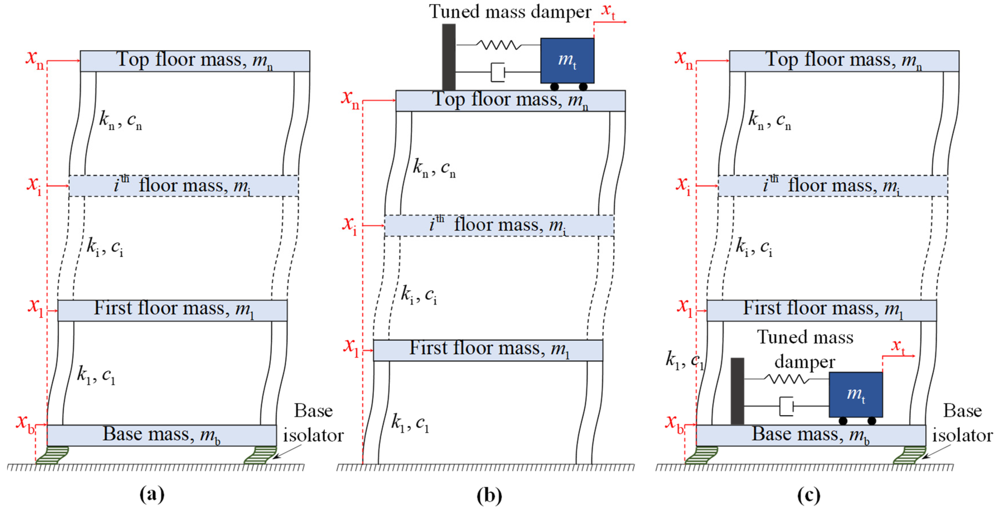
A TMD is a large mass (hundreds of tons) connected to the building with springs and dampers. The entire system—building + TMD—is a coupled oscillator. The TMD is "tuned" so that its own natural frequency is very close to the building's primary resonant frequency. When the building starts to sway at its resonant frequency, the TMD begins to oscillate with a large amplitude, 180 degrees out of phase with the building's motion. This counter-oscillation exerts a force on the building that opposes its sway, effectively absorbing the vibrational energy and damping the motion. The massive pendulum in the Taipei 101 skyscraper is a famous example of a TMD.

Challenge Problem

To solidify your understanding, here is a problem at the level you're aiming for. It guides you through the complete analysis of a different coupled system: two masses connected by three springs.

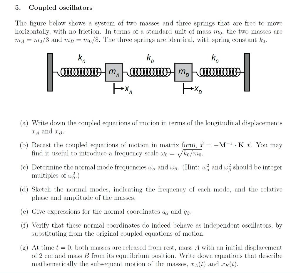
Try to work through parts (a) through (d) using the eigenvalue method we developed today.

Conclusion

Today, we made the leap from single oscillators to coupled systems. This introduced a new layer of complexity but also revealed an underlying simplicity in the form of normal modes.

Key Takeaways:

• Coupled oscillators are systems where the motion of individual components is interdependent, leading to coupled differential equations.
• Normal modes are special collective oscillation patterns where all parts of the system move harmonically with the same, single normal frequency.
• The general motion of any coupled system is a superposition of its normal modes.
• We can find the normal frequencies and mode shapes by recasting the equations of motion in matrix form ($M\ddot{X}=-KX$) and solving the resulting eigenvalue problem, $(M^{-1}K)A={\omega }^{2}A$.
• The normal frequencies are found by solving the characteristic equation $\det (K-{\omega }^{2}M)=0$.

Preview of the Next Lesson:
We've analyzed a system with two degrees of freedom. What happens when we have three, four, or even an infinite number of coupled oscillators? In our next lesson, we will analyze a chain of many coupled masses. As we take the limit where the number of masses becomes infinite and their separation becomes infinitesimal, our system of coupled oscillators will transform into a continuous medium. This will lead us directly to the derivation of the wave equation, bridging the gap between discrete mechanics and continuum mechanics.