Hello! In our last lesson, we took a major step toward modeling real-world oscillators by introducing damping. We saw how the homogeneous equation led to three distinct behaviors—underdamped, overdamped, and critically damped—that describe how a system naturally comes to rest.
Today, we complete our model by adding the final, crucial ingredient: an external driving force. This will allow us to analyze driven, damped harmonic oscillators, derive the conditions for resonance, and apply these concepts to engineering systems. We'll see what happens when a system is no longer left to itself but is instead forced to oscillate by an external agent. This leads to the phenomenon of resonance, one of the most fundamental and ubiquitous concepts in all of physics and engineering, governing everything from tuning a radio to the structural integrity of a bridge.
1. The Equation of Motion and the Steady-State Solution
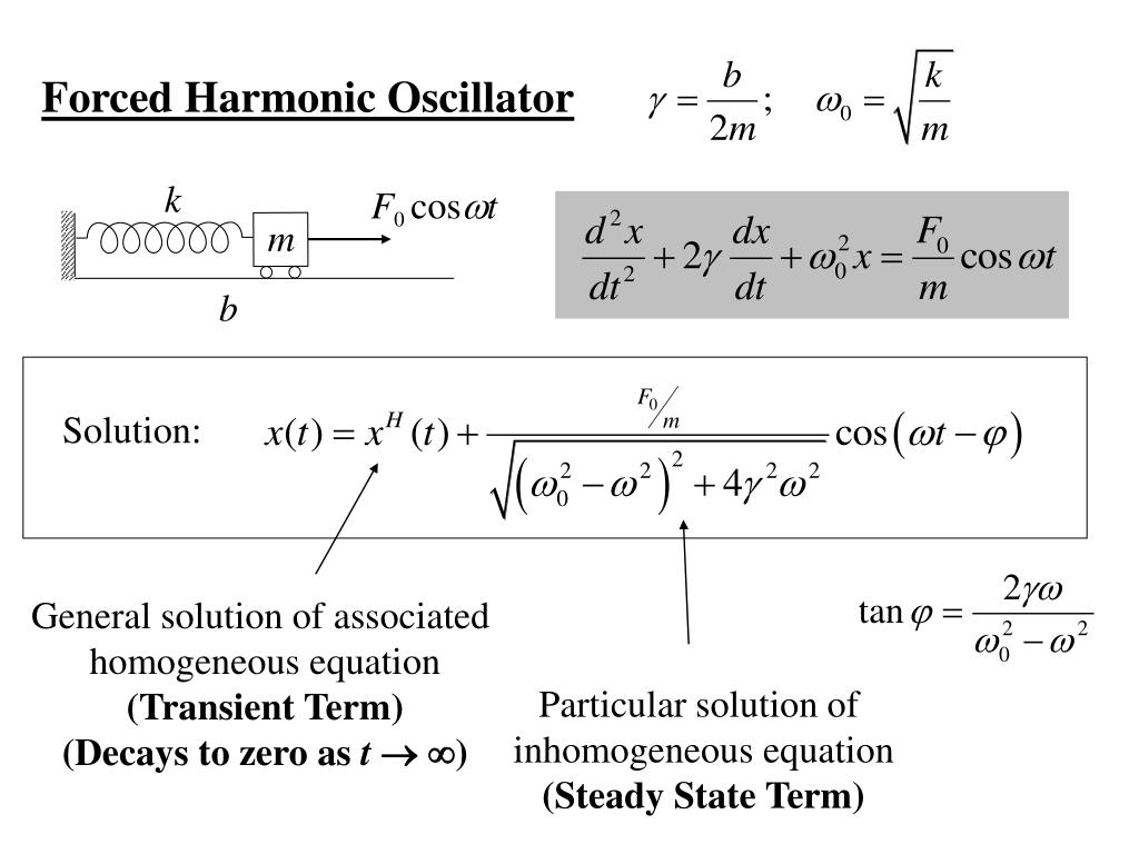
We begin with our damped oscillator and now apply an external, sinusoidally varying force, which we can write as . Here, is the force amplitude and is the driving angular frequency, which is completely independent of the oscillator's natural frequency, .
Applying Newton's second law, , gives:
Rearranging and using our established definitions, and , we get the governing equation for a driven, damped harmonic oscillator:
This is a linear, second-order, inhomogeneous differential equation. Its solution has two parts:
- The transient solution (), which is the solution to the homogeneous equation we studied last lesson. This part depends on the initial conditions and decays exponentially over time.
- The steady-state solution (), a particular solution that describes the system's long-term behavior, oscillating at the driving frequency .
Initially, the motion is a complex superposition of both, but eventually, the transient part dies out, leaving only the steady-state motion. Our primary goal is to find and analyze this steady-state solution.
The following video provides an outstanding derivation of the steady-state solution. Professor Lewin uses complex numbers to solve the differential equation, a powerful technique that elegantly handles both amplitude and phase.
8.03 - Lect 3 - Driven Oscillations With Damping, Steady State Solutions, Resonance
Watch this lecture by Prof. Walter Lewin from MIT. He introduces the driven oscillator, sets up the differential equation, and uses complex exponentials to find the steady-state solution. This method is mathematically robust and provides great physical insight.
Please watch from the beginning to 9:52. The video will first set up the equation (0:06-2:09), then propose a complex trial solution to find the steady-state response (2:09-6:42), and finally solve for the amplitude and phase lag (6:42-9:52).
As derived in the video, the steady-state solution has the form:
The system oscillates at the driving frequency , but with an amplitude and a phase lag that depend on . The expressions for and are:
- Amplitude:
- Phase Lag:
These two equations are the core of our analysis. For a clear, textual summary of this derivation and the resulting formulas, you can refer to the resource PPLATO | FLAP | PHYS 5.3.
PPLATO | FLAP | PHYS 5.3: Forced vibrations and resonance
This text from the PPLATO project provides a rigorous, step-by-step derivation of the amplitude and phase lag equations. It's a great written companion to the video's derivation.
Read 'Section 2.3 Steady state motion'. Focus on how the trial solution (Equation 9) is substituted into the differential equation to yield expressions for the amplitude (Equation 15) and phase lag (Equation 16).
2. Analysis of the Steady-State Response: Resonance
Now, let's analyze the behavior of the amplitude and phase lag at different driving frequencies.
Limiting Cases
Professor Lewin's video provides excellent physical intuition for the behavior at extreme frequencies.
8.03 - Lect 3 - Driven Oscillations With Damping, Steady State Solutions, Resonance
Let's return to Prof. Lewin's lecture, where he masterfully interprets the amplitude and phase equations we've just derived in different frequency regimes.
Watch the segment from 9:52 to 18:22. Pay close attention to his physical reasoning for the system's behavior in three key cases: very low frequency (\Omega o 0), resonance (\Omega = \omega_0), and very high frequency (\Omega o \infty).
To summarize the key points:
-
Low Driving Frequency ():
- Amplitude: . The spring is simply following the slowly applied force.
- Phase Lag: . The displacement is in phase with the driving force.
-
High Driving Frequency ():
- Amplitude: . The mass's inertia prevents it from keeping up with the rapid oscillations of the force.
- Phase Lag: approaches 0 from the negative side, meaning (180°). The displacement is completely out of phase with the force.
-
Resonance ():
- Amplitude: The term becomes zero, and the amplitude reaches its maximum value (or close to it): .
- Phase Lag: The denominator of is zero, so (90°). The displacement lags the force by a quarter of a cycle.
This dramatic increase in amplitude when the driving frequency is close to the natural frequency is known as resonance. The sharpness and height of this resonance peak are determined by the amount of damping, which we often characterize by the Quality Factor (Q-factor), where for light damping . A high-Q system (low damping) has a very tall and narrow resonance peak.

Test your understanding!
Consider a driven, damped oscillator with mass kg, spring constant N/m, and damping coefficient N·s/m. It is driven by a force .
- Calculate the natural frequency and the damping constant .
- Calculate the amplitude of oscillation at resonance ().
- Calculate the amplitude of oscillation when driven at a very low frequency ().
- By what factor is the amplitude at resonance larger than the low-frequency amplitude? How does this relate to the Q-factor?
Show answer
-
rad/s.
s⁻¹. -
At resonance, m.
-
At low frequency, m.
-
The ratio is . The Q-factor is . For a lightly damped system, the amplitude at resonance is approximately Q times the amplitude at very low frequency.
3. Transient Behavior and Power Absorption
As mentioned earlier, the steady-state solution is only what's left after a long time. The complete solution is the sum of the transient and steady-state parts.
When you first turn on the driving force, the system tries to oscillate at its own damped natural frequency while also being forced at frequency . The initial motion is a combination of these two, which can lead to complex behavior like beats if is close to .
The following video demonstrates this beautifully and then transitions into a discussion of the energy required to sustain the oscillation.
8.03 - Lect 4 - Forced Oscillations, Power, Resonance, Transient Solutions
This second lecture from Prof. Lewin starts by explaining and demonstrating the transient solution and the beats phenomenon. It then provides a rigorous derivation for the average power absorbed by the oscillator, showing that power absorption is maximized at resonance.
Please watch the following segments: Transient Behavior (0:06 - 20:18): Focus on the concept of the general solution being the sum of the transient and steady-state parts. The demonstration starting around 15:33 vividly shows the transient beats before settling into the steady state. Power Absorption (20:18 - 39:39): Follow the derivation of the average power (\langle P angle) supplied by the driver. Note that this power is used to counteract the energy dissipated by the damping force. The key result is understanding how (\langle P angle) changes with frequency and that it peaks exactly at \Omega = \omega_0. This is power resonance.
Power Resonance
The driver must do work to counteract the energy dissipated by the damping force. The instantaneous power delivered by the driver is . The average power delivered over one cycle, , is what sustains the oscillation.
As derived in the video and the PPLATO text (LINK, Section 2.4), the average power absorbed by the oscillator is:
Substituting the expression for gives a formula for power as a function of frequency. The most important result is that this power absorption is maximized at resonance (), where it reaches:
The width of this power-resonance curve (specifically, the "full width at half maximum," or FWHM) is given by . This leads to a fundamental relationship:
This shows that a high-Q system not only has a large amplitude response but also a very sharp and selective frequency response for absorbing power.
4. Applications in Engineering and Physics
The principles of driven oscillations and resonance are universal. Here are a few key applications.
RLC Circuits: A Perfect Analogy
Your background in electricity and magnetism will make this analogy particularly insightful. An RLC circuit (a circuit with a resistor, inductor, and capacitor) driven by an AC voltage source is the direct electrical analogue of a driven mechanical oscillator.
| Mechanical System | Electrical System |
|---|---|
| Position, | Charge, |
| Velocity, | Current, |
| Mass, (Inertia) | Inductance, |
| Damping, | Resistance, |
| Spring Constant, | Inverse Capacitance, |
| Driving Force, | Driving Voltage, |
The differential equation for the charge in an RLC circuit is:
This is mathematically identical to the mechanical oscillator's equation. The natural frequency is , and resonance occurs when the driving frequency matches this, leading to a large current in the circuit. This is precisely how you tune a radio: you change the capacitance or inductance of a circuit to make its resonant frequency match the frequency of the radio station you want to receive.
8.03 - Lect 4 - Forced Oscillations, Power, Resonance, Transient Solutions
Let's watch the segment from Prof. Lewin's lecture where he explicitly makes this connection to RLC circuits and demonstrates electrical resonance.
Watch from 40:22 to 1:00:35. Notice how he derives the identical differential equation and predicts the behavior of the current at resonance. The oscilloscope demonstration provides clear, quantitative proof of the resonance theory.
Other Examples of Resonance
- Mechanical Systems: Pushing a child on a swing (you time your pushes to match the swing's natural frequency), the rattling of a car part at a specific engine RPM, or the catastrophic collapse of the Tacoma Narrows Bridge in 1940, where wind provided a driving frequency that matched one of the bridge's natural frequencies.
- Acoustic Systems: A singer shattering a crystal glass by matching its resonant frequency with a sustained, powerful note.
- Atomic & Quantum Systems: Atoms and molecules absorb light (electromagnetic radiation) only at specific resonant frequencies corresponding to their internal energy levels. This is the basis of all spectroscopy, which allows us to determine the chemical composition of stars. Professor Lewin's demonstrations with tuning forks and sodium vapor are beautiful examples of this principle.
Conclusion
In this lesson, we have fully characterized the behavior of a damped oscillator under the influence of a periodic driving force. We moved from a homogeneous to an inhomogeneous differential equation and saw how this introduced the concepts of transient and steady-state behavior.
Key Takeaways:
- A driven, damped oscillator is governed by the equation .
- After initial transients die out, the system enters a steady state, oscillating at the driving frequency .
- Resonance is the phenomenon where the system's response amplitude is maximized when the driving frequency is close to the natural frequency .
- At resonance, the phase lag between the driving force and the displacement is 90°.
- The driver supplies power to counteract damping. The rate of power absorption also peaks sharply at resonance.
- The Q-factor () determines the sharpness of the resonance: high-Q systems have very tall, narrow resonance peaks, making them highly selective in frequency.
- The principle of resonance is fundamental across physics and engineering, with direct analogues in mechanical, electrical, and even quantum systems.
Preview of the Next Lesson:
We have now mastered the behavior of a single oscillator. The next logical step is to see how multiple oscillators interact with each other. In the next lesson, we will begin our study of coupled oscillators, where the motion of one oscillator influences the motion of another. This will introduce the powerful concept of normal modes, which are the collective oscillation patterns of a system.