Transient and Steady-State Analysis of RLC Circuits using ODEs

1. First-Order Circuits: The Transient Response

First-order circuits contain one energy storage element (either an inductor or a capacitor) and a resistor. Their behavior is described by a first-order linear ODE. Let's analyze the case where a DC voltage source is suddenly connected to the circuit.

The solution to these ODEs has two parts:

1. The Homogeneous Solution (Transient Response): This part describes how the circuit naturally returns to equilibrium. It always decays exponentially to zero.
2. The Particular Solution (Steady-State Response): This part describes the circuit's behavior after a long time has passed. For a DC source, it's the final, stable state.

The total solution is the sum of these two parts, with constants determined by the initial conditions of the circuit.

The RC and RL Circuits with a DC Source

Let's watch a video that derives and solves the governing ODEs for both RC and RL circuits when a DC voltage is applied. This will formalize the concepts of charging/discharging and the time constant.

As the video demonstrated, the governing equations are:

• RC Circuit: $R\frac{dQ}{dt}+\frac{1}{C}Q=V_s⟹\frac{d{V}_C}{dt}+\frac{1}{RC}{V}_C=\frac{V_s}{RC}$
• RL Circuit: $L\frac{dI}{dt}+RI=V_s$

In both cases, the transient part of the solution decays as $e^{-t/\tau }$, where the time constant $\tau$ determines the speed of the decay:

• For an RC circuit, $\tau =RC$.
• For an RL circuit, $\tau =L/R$.

After about $5\tau$, the transient response becomes negligible, and the circuit is considered to have reached its steady state.

2. Second-Order Circuits: The Series RLC Circuit

Now, let's add all three components—R, L, and C—in series with a voltage source $V_s$. This creates a second-order system with richer and more complex behavior.

Applying Kirchhoff's Voltage Law (KVL) around the loop gives:

Substituting the V-I relationships $V_L=L\frac{dI}{dt}$, $V_R=IR$, and $I=\frac{dQ}{dt}$ (so $V_C=Q/C$), we get:

This is a second-order, linear, inhomogeneous ordinary differential equation. You should immediately recognize its form. It is mathematically identical to the equation for a damped, driven mechanical oscillator:

This is not just a coincidence; it's a deep physical analogy:

• Inductance ($L$) acts like mass ($m$): It represents inertia, resisting changes in current (velocity).
• Resistance ($R$) acts like damping ($b$): It dissipates energy.
• Inverse Capacitance ($1/C$) acts like the spring constant ($k$): It stores potential energy.
• Charge ($Q$) is analogous to position ($x$), and Current ($I$) is analogous to velocity ($v$).

The Transient Response of an RLC Circuit

The transient behavior is described by the homogeneous equation (setting $V_s=0$). We solve this by substituting an ansatz $Q(t)=e^{rt}$, which yields the characteristic equation:

The roots of this quadratic equation determine the nature of the transient response:

Just as with a mechanical oscillator, we have three distinct regimes depending on the values of R, L, and C.

To formalize this, we define two important parameters:

• Damping Factor: $\alpha =\frac{R}{2L}$
• Natural (Resonant) Frequency: ${\omega }_0=\frac{1}{\sqrt{LC}}$

The roots can then be written as $r=-\alpha \pm \sqrt{{\alpha }^2-{\omega }_0^2}$.

The following video provides an excellent and comprehensive derivation of these three cases.

Let's summarize the three cases discussed in the video:

1. Overdamped ($\alpha >{\omega }_0$):
   • Condition: $(\frac{R}{2L}{)}^2>\frac{1}{LC}$ or $R>2\sqrt{\frac{L}{C}}$.
   • The characteristic equation has two distinct, real, negative roots.
   • The solution is a sum of two decaying exponentials: $Q_h(t)=c_1{e}^{r_{1}t}+c_2{e}^{r_{2}t}$.
   • The system returns to equilibrium slowly and without any oscillation.

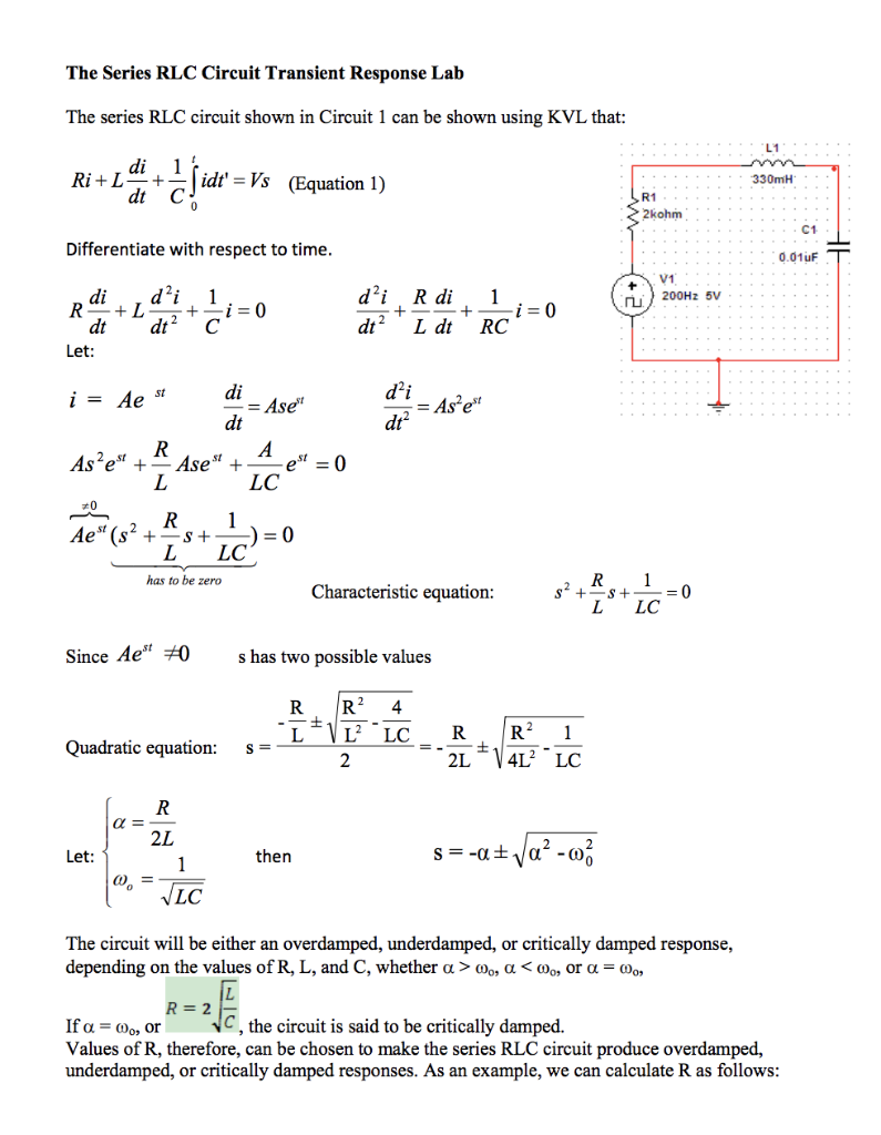
*This image shows the derivation of the RLC equation and the conditions for the three damping regimes, providing a concise mathematical summary.*

2. Critically Damped ($\alpha ={\omega }_0$):
* Condition: $(\frac{R}{2L}{)}^2=\frac{1}{LC}$ or $R=2\sqrt{\frac{L}{C}}$.
* The characteristic equation has one repeated, real, negative root ($r=-\alpha$).
* The solution has the form: $Q_h(t)=(c_1+c_{2}t)e^{-\alpha t}$.
* This is the "sweet spot" that provides the fastest return to equilibrium without any overshoot or oscillation. This is highly desirable in many engineering applications, like the suspension in a car or a closing automatic door.

3. Underdamped ($\alpha <{\omega }_0$):
   • Condition: $(\frac{R}{2L}{)}^2<\frac{1}{LC}$ or $R<2\sqrt{\frac{L}{C}}$.
   • The characteristic equation has two complex conjugate roots: $r=-\alpha \pm i{\omega }_d$, where ${\omega }_d=\sqrt{{\omega }_0^2-{\alpha }^2}$ is the damped frequency.
   • The solution is a decaying sinusoid: $Q_h(t)=e^{-\alpha t}(A\cos ({\omega }_{d}t)+B\sin ({\omega }_{d}t))$.
   • The system oscillates as it returns to equilibrium, with the amplitude of oscillations decaying exponentially. This is the behavior seen in radio tuners and filters.

*This image visually summarizes the underdamped case, showing the circuit, the governing equation, the form of the solution, and the characteristic decaying oscillatory waveform.*

3. Mathematical Rigor: The ODE Solution Method

Your preference for mathematical rigor is well-served by a deeper look into solving these ODEs. The text "Differential Equations for Engineers" provides a formal treatment that parallels our circuit analysis.

This reading confirms that the method for analyzing RLC circuits is a direct, robust application of the theory of ordinary differential equations.

4. Parallel RLC Circuits

The same principles apply to a parallel RLC circuit, but the analysis starts with Kirchhoff's Current Law (KCL). The resulting ODE has a similar second-order form, but the roles of R, L, and C in the coefficients are different. For instance, in a parallel circuit, a large resistance leads to less damping, because less current is diverted through the dissipative path. You can find a detailed derivation in the video "Transient Analysis of the RLC Circuit" from 13:21 to 18:43.

5. Solving a Complete Problem

Let's see how to solve for the transient current in a circuit, including finding the unknown constants using initial conditions. The initial conditions are based on the principles that:

• Inductor current cannot change instantaneously: $I_L(0^{-})=I_L(0^{+})$.
• Capacitor voltage cannot change instantaneously: $V_C(0^{-})=V_C(0^{+})$.

Watch one of the worked examples from the video we saw earlier.

Conclusion

In this lesson, we have seen how the principles of circuit theory and differential equations combine to provide a complete description of RL, LC, and RLC circuits.

Key Takeaways:

• The behavior of RLC circuits is governed by second-order linear ODEs, which are analogous to the equations of a damped mechanical oscillator.
• The transient response is the solution to the homogeneous ODE and decays over time. Its character depends on the circuit's components.
• The three regimes of transient response are overdamped (slow, non-oscillatory decay), critically damped (fastest non-oscillatory decay), and underdamped (decaying oscillations).
• The steady-state response is the particular solution to the inhomogeneous ODE and describes the circuit's long-term behavior.
• The complete solution is the sum of the transient and steady-state responses, with constants determined by initial conditions.

Preview of the Next Lesson:
Our analysis today focused on the "lumped element" model, where fields are confined to ideal components. However, this model has its limits. A key piece is missing from Ampere's Law when fields are changing in time. In our next lesson, "Formulate the Ampère-Maxwell law by introducing the concept of displacement current," we will address this inconsistency. This will complete the full set of Maxwell's equations and pave the way for understanding one of the most profound discoveries in physics: electromagnetic waves.