Welcome back! In our previous lesson, you mastered the VLOOKUP function and, just as importantly, learned to recognize its significant limitations. We saw that it can't look to its left and that its reliance on a fixed column index number makes formulas fragile. This critical understanding sets the stage for what comes next.
Today, you will learn the classic and powerful solution to these problems: the INDEX and MATCH functions. By combining these two, you can create lookups that are more flexible, robust, and capable than VLOOKUP. We will deconstruct the lookup process into two distinct steps, learn how each function works individually, and then combine them to overcome all of VLOOKUP's major weaknesses.
Deconstructing the Lookup: From VLOOKUP to INDEX and MATCH
VLOOKUP performs two actions in one step: it finds the correct row and then retrieves a value from a specified column in that row. The power of INDEX and MATCH comes from separating these two actions.
MATCH: This function's only job is to find the position of an item in a list. It answers the question, "In which row (or column) number is my item located?"INDEX: This function's job is to retrieve a value from a specific location (or "coordinate") within a range. It answers the question, "What value is in the 5th row and 2nd column of this table?"
By using MATCH to find the coordinates and feeding them to INDEX, we can build a superior lookup formula.
Let's start by understanding each function on its own. The article "Excel INDEX MATCH vs. VLOOKUP" from Ablebits provides a great introduction.
Excel INDEX MATCH vs. VLOOKUP - formula examples
This reading will introduce you to the syntax and purpose of the INDEX and MATCH functions separately, before we combine them.
First, read the section about the INDEX function. Focus on how it uses row and column numbers to retrieve a value from an array. Next, read the section on the MATCH function. Notice that its purpose is simply to return the relative position of an item. Pay attention to the third argument, match_type, which should be 0 for an exact match, just like FALSE in VLOOKUP. Finally, read the short section on how they work together to get a high-level overview.
Building the INDEX and MATCH Formula
Now that you have a basic understanding of what INDEX and MATCH do, let's see them in action. The best way to learn this is to watch an expert build the formula from scratch.
How to use Excel Index Match (the right way)
This video by Leila Gharani provides an excellent, step-by-step demonstration. She uses a clear analogy of INDEX being a "GPS" that needs coordinates, which MATCH provides.
First, watch the explanation of INDEX on its own from this section. Notice how it returns a value based on hard-coded row and column numbers. Next, see how MATCH works from this part. The key insight is that it returns the number that INDEX needs for its row argument. Finally, watch how she combines INDEX and MATCH to create a dynamic lookup from this demonstration. Pay close attention to the formula structure: =INDEX(column_to_return_from, MATCH(what_to_find, where_to_find_it, 0)). Notice how the ranges for INDEX and MATCH must have the same height to stay in sync.
The combination you just saw, INDEX(MATCH), directly solves the two main problems of VLOOKUP:
- Left Lookup: Because you specify the lookup column and return column as two separate ranges, their relative positions don't matter. You can easily look up a value in column
Cand return the corresponding value from columnA. - Robustness: The formula refers to the entire columns, not a hard-coded index number. If you insert or delete columns between your lookup and return columns, the formula will not break.
Two-Way Lookups with INDEX and MATCH MATCH
The flexibility of this combination allows for even more powerful lookups. What if you need to find a value based on criteria in both a row and a column? This is called a two-way or matrix lookup. For example, finding the sales for a specific employee (row) in a specific month (column).
To achieve this, we simply use a second MATCH function to find the column number.
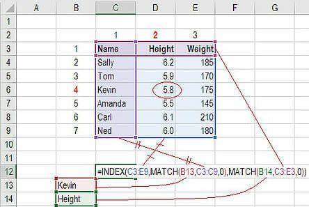
The structure becomes:=INDEX(table_of_values, MATCH(row_lookup_value, row_headers, 0), MATCH(column_lookup_value, column_headers, 0))
Let's continue with the video to see how this is done.
How to use Excel Index Match (the right way)
This segment demonstrates the powerful two-way lookup.
Watch from this section where the formula is expanded to make both the row and column dynamic. Notice how one MATCH provides the row number and a second MATCH provides the column number.
This image provides a great visual breakdown of how the INDEX(MATCH, MATCH) formula works. Each MATCH function finds a coordinate, and INDEX retrieves the value at their intersection.
For a written explanation and another example of this powerful technique, you can review the Ablebits article again.
Excel INDEX MATCH vs. VLOOKUP - formula examples
This section of the Ablebits article provides a detailed text-based breakdown of a two-way lookup formula.
Read the section titled INDEX MATCH MATCH. Follow the logic of how the formula is broken down into its three main parts.
A Common Pitfall: Misaligned Ranges
The most common error when using INDEX and MATCH is the #REF! error. This usually happens when the size of the array in the INDEX function does not match the size of the lookup array in the MATCH function.
For example, if your INDEX array is C2:C10 (9 rows) but your MATCH lookup array is A2:A12 (11 rows), the formula can produce an error. If MATCH finds a result in the 10th position of its range, it will pass the number 10 to INDEX. However, the INDEX range only has 9 rows, so it can't find the 10th item, resulting in an error.
Always ensure your row ranges have the same number of rows.

The Excel Campus video provides a great explanation of this common issue.
How To Use Index Match As An Alternative To Vlookup
This video segment explains the cause of the most common error you'll encounter with INDEX MATCH.
Watch the section from 15:14 to 17:13 to understand how mismatched range sizes cause the #REF! error and see a real-world example of how this can happen.
Conclusion
You have now added an incredibly powerful and flexible tool to your Excel skillset. While VLOOKUP is common, mastering INDEX and MATCH is what separates intermediate users from advanced practitioners. You can now build lookups that are more reliable and can handle far more complex scenarios.
Here are the key takeaways from this lesson:
- Separate Functions, More Power:
INDEXretrieves a value by its coordinates, whileMATCHfinds the coordinates. Separating these actions is the key to its flexibility. - One-Way Lookup: The formula
=INDEX(return_range, MATCH(lookup_value, lookup_range, 0))overcomesVLOOKUP's main limitations. It can look left and is not broken by inserting/deleting columns. - Two-Way Lookup: The formula
=INDEX(data_table, MATCH(row_value, row_range, 0), MATCH(col_value, col_range, 0))allows you to perform dynamic lookups in a matrix or grid. - Range Alignment is Crucial: Always ensure the array ranges in your
INDEXandMATCHfunctions are properly aligned and have the same number of rows (for vertical lookups) to avoid errors.
In our next lesson, we will explore XLOOKUP. This is a modern function available in newer versions of Excel that combines the power of INDEX and MATCH into a single, easier-to-use function, officially succeeding VLOOKUP.