Forecasting Revenue and Expenses with Assumptions

1. The Core Drivers of a Forecast

Before we write any formulas, let's establish the basic logic. A financial forecast is simply a mathematical representation of a business's operations. At its simplest, this can be broken down into three core components, which are clearly defined in the following resource.

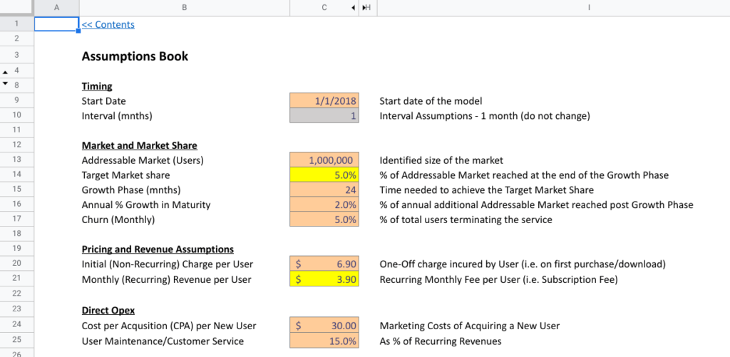
These three equations are the "physics" of our model. The variables within them—quantity, price, fixed costs, and variable costs—are called drivers. Our assumptions section is where we will define and control these drivers.

2. Building the Revenue Forecast

With the theory in place, let's start building. Our first task is to project revenue. We will do this by defining our drivers (e.g., number of orders, price per order, and growth rate) in the assumptions section and then using formulas in the main statement to calculate the revenue for each forecast period.

The following video provides a clear, practical demonstration of this process.

This process creates a dynamic link. If you change the 'Order Growth Rate' in the assumptions, the 'Number of Orders' and, consequently, the 'Revenue' will update automatically. This is the flexibility clients pay for.

The "Financial Forecasting Guide" from the Corporate Finance Institute reinforces this with explicit formulas. For a year-over-year growth model, the formula for the first forecast year's sales is:

=C42*(1+D8)

Where C42 is the previous year's sales and D8 is the sales growth assumption. This is precisely the logic applied in the video.

3. Building the Expense Forecast

Next, we'll forecast the costs. As we learned from our reading, costs come in two main flavors: variable and fixed.

• Variable Costs are often grouped into the Cost of Goods Sold (COGS). These costs scale directly with revenue or quantity. For example, the cost of manufacturing a t-shirt is incurred for every t-shirt sold.
• Fixed Costs are typically called Operating Expenses (OPEX) or SG&A (Selling, General & Administrative). These are the costs of being in business, regardless of sales volume, such as rent, salaries, and marketing budgets. In reality, these can change over time (e.g., hiring more staff as you grow), so we model them as "steps" in our forecast.

Let's return to the video to see how to model both types.

An Alternative Method: Percentage of Sales

Another extremely common method for forecasting expenses, especially SG&A, is to assume they will represent a certain percentage of sales. This is particularly useful when you don't have detailed per-unit cost information but have historical data suggesting a stable relationship between sales and expenses.

The CFI "Financial Forecasting Guide" provides the perfect formula for this. To calculate an expense line like "Distribution Expenses" as a percentage of sales, you would use:

=D$42*D10

Here, D$42 refers to the Sales for the current period, and D10 refers to the assumption for "Distribution Expense as a % of Sales". The dollar sign $ creates a mixed reference. As you drag this formula down to calculate other expenses (like Marketing or Depreciation), the reference to the expense assumption (D10) will change, but the reference to the sales row ($42) will remain locked. This is an efficient technique you learned about back in Module 1.

4. Putting It All Together

You have now built the core components of your forecast: a revenue projection and an expense projection, both dynamically driven by a centralized assumptions section. Your simplified income statement structure might now look something like the example below, with each of the forecast numbers being the result of a formula.

By following the principles from today's lesson, you have created a model where you can ask "what-if" questions simply by changing a number in the assumptions section and watching the entire forecast update instantly.

Conclusion

Today you've transitioned from architect to builder, putting the structural theory from our last lesson into practice. You've constructed the essential revenue and expense forecasts that form the engine of a financial model, ensuring every projection is traceable to a clear assumption.

Key Takeaways:

• Forecasts are built on drivers: Revenue and expenses are driven by key business variables like quantity, price, and costs, which are defined in your assumptions section.
• Revenue Forecasting: A common method is to project a primary driver (like Number of Orders) based on a growth rate, then multiply it by a secondary driver (like Price per Order).
• Expense Forecasting: Costs are separated into variable (COGS), which scale with quantity, and fixed (OPEX), which are modeled as fixed amounts that can step up over time. Forecasting expenses as a percentage of sales is also a powerful technique.
• Dynamic Linking is Key: The power of a financial model comes from using formulas to link your outputs (the forecast) to your inputs (the assumptions), creating a flexible and auditable tool.

In our next lesson, we will complete our initial financial statement. With revenue and expenses forecasted, we will consolidate these projections to calculate essential profit metrics like Gross Profit, EBITDA, and Net Income, giving us a full top-to-bottom view of the company's projected profitability.