Introduction
In our last lesson, we focused on combining data vertically by appending tables together. This is a crucial skill for consolidating data from multiple sources. Now, we shift our attention from combining tables to reshaping the data within a single table. You will often receive data that is structured for easy human reading but is difficult for Excel to analyze. This is commonly known as "wide" or "crosstab" data.
This lesson will teach you how to use one of Power Query's most transformative features: Unpivot Columns. This tool allows you to take wide data, where values are spread across multiple columns (like sales for Jan, Feb, Mar, etc.), and transform it into a "tidy" or "tall" format. In a tidy format, each observation has its own row, making it perfect for analysis with PivotTables, charts, and other Excel tools. Mastering this will dramatically increase the efficiency of your data preparation work.
1. Understanding "Wide" vs. "Tidy" Data
Before we jump into the mechanics, it's essential to understand the problem we're solving. Most data can be structured in two ways:
- Wide Data: This format is often a summary or a report. It's easy for a person to scan across columns. A classic example is a sales report with products listed in rows and months listed as separate columns. While readable, this structure is inflexible for analysis. How would you filter for all sales in Q1? Or create a chart showing sales trends over 24 months? It would be very manual.
- Tidy Data: In this format, each column represents a distinct variable (e.g., Product Name, Date, Sales Amount), and each row represents a single observation (e.g., the sales for one product on one date). This structure is the gold standard for data analysis and is what tools like PivotTables expect.
The image below illustrates this transformation perfectly. The table on the left is a "wide" report. The table on the right is the same data in a "tidy," analysis-ready format. The Unpivot operation is what makes this change possible.
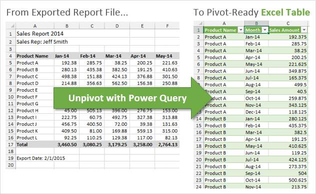
To grasp why this is so fundamental, let's look at the official Microsoft documentation which explains the problem and the goal.
This article from Microsoft Learn provides a clear, concise explanation of the unpivoting concept.
Read the introductory section, starting from the beginning down to the key concept. Notice how the "before" table is hard to filter by date, while the "after" table makes it simple. This is the core reason we unpivot data.
2. How to Unpivot Data in Power Query
Now that you understand the "what" and "why," let's focus on the "how." The process is surprisingly straightforward and, because it's in Power Query, completely repeatable.
We will watch a video that walks through a complete example, from loading the data to outputting the final tidy table. The video also highlights an important side benefit: Power Query automatically removes blank or null values during the unpivot process, cleaning your data as it reshapes it.
How to Unpivot Data with Power Query in Excel
This video from Excel Campus provides a thorough walkthrough of the entire unpivoting process, including best practices.
Please watch from the beginning to the loading step. The presenter covers the essential steps: Defining the Goal: A clear visual of the desired transformation (00:00 - 00:38). Loading to Power Query: Converting the range to an Excel Table and loading it into the editor (00:53 - 01:25). Unpivoting: Selecting the data columns (Apples through Tea) and clicking the Unpivot Columns button (01:25 - 01:58). Renaming Columns: Renaming the default 'Attribute' and 'Value' columns to something meaningful, like 'Product' and 'Quantity' (01:58 - 03:20). Loading to Excel: Using Close & Load to place the new, tidy table in a worksheet (03:20 - 03:38).
A key takeaway from the video is the renaming step. Power Query will always name the two new columns 'Attribute' (for the former column headers) and 'Value' (for the values within the cells). You should always rename these to be descriptive of your actual data.
3. Choosing the Right Unpivot Strategy
In the video, the presenter selected all the columns he wanted to unpivot. However, Power Query gives you three distinct options, and choosing the right one is key to building robust queries that don't break when your source data changes.

Let's explore these options using the Microsoft documentation.
This part of the documentation clearly explains the three methods and, most importantly, how each behaves when new data is added to your source file upon refresh.
Please read the following three sections: Unpivot Columns: This is the method where you select the columns to transform. Notice that if a new date column is added to the source, it gets unpivoted too. Unpivot Other Columns: Here, you select the columns to keep (e.g., an ID or category column), and Power Query unpivots everything else. This is generally the most robust method because it automatically handles new columns added in the future (like a new month's sales data). Unpivot Only Selected Columns: This is a more explicit version of the first method. It will only unpivot the columns you originally selected and will ignore any new columns added later.
For most of your freelance work, Unpivot Other Columns will be your best choice. It makes your solution dynamic. If a client adds a new month or a new product category as a column to their source file, you only need to refresh your query, and the new data will be correctly transformed and included without you having to edit the query steps.
4. Practice and Automation
Now it's time to put this into practice. The true power of this technique lies in its automation. Once you set up the query, you can add new data to your source table, click refresh, and your tidy output table will update instantly.
The video you watched earlier demonstrates this refresh capability.
How to Unpivot Data with Power Query in Excel
Let's revisit the Excel Campus video to see the automation in action.
Watch the final segment from 03:44 to 04:51, where the presenter adds a new row and a new column to the source data. Notice how a simple right-click and Refresh on the output table is all that's needed to incorporate the new data.
To solidify your understanding, here is a practical exercise with a downloadable file. Applying the steps you've just learned is the best way to make them stick.
Unpivot columns using Power Query
This page from Excel Practice Online provides a chance for hands-on practice.
Navigate to the section Practice Unpivot. Download the provided exercise file and use the Unpivot feature in Power Query to transform the tourism data into a tidy format. Try to use the Unpivot Other Columns method.
Conclusion
In this lesson, you've added a powerful data-shaping tool to your Power Query arsenal. You learned the critical difference between wide and tidy data and now understand why tidy data is essential for analysis. Most importantly, you can now use the Unpivot feature to perform this transformation efficiently and automatically.
Key Takeaways:
- Wide vs. Tidy: Wide data is for human readability; tidy data is for machine analysis. Your goal is usually to get data into a tidy format.
- Unpivot is the Tool: Power Query's
Unpivot Columnsfeature is the primary way to transform wide data into tidy data. - Choose the Right Strategy: For queries that need to adapt to future data,
Unpivot Other Columnsis typically the most robust and flexible choice. - Automate and Refresh: The entire transformation is recorded as a query step, allowing you to simply refresh your output when the source data changes, saving you enormous amounts of time.
You've now learned how to combine data (Append and Merge) and how to reshape it (Unpivot). In our next lesson, we will build directly on the tidy data format you learned to create today. We will explore how to group and aggregate data within the Power Query editor, allowing you to perform calculations and create summary tables before the data even reaches Excel.