Welcome to your next lesson in data preparation. In our previous session, we focused on sorting, which is about rearranging all of your data to bring order to it. Now, we'll explore a complementary and equally vital skill: filtering.
While sorting reorders your entire dataset, filtering allows you to temporarily hide the rows you don't need, letting you focus intensely on a specific subset of your information. Imagine a client gives you a sales report for the entire year and asks, "How did our top products perform in the last quarter in the North region?" Answering this question efficiently is impossible without filtering.
This lesson will teach you how to use Excel's AutoFilter tool. You will learn to extract specific data based on text, numbers, dates, and even cell formatting. Mastering this is a fundamental step in data cleaning and analysis, a core competency for any freelance Excel professional.
Activating Filters and Basic Selection
The AutoFilter feature adds a small dropdown arrow to the header of each column in your dataset. Clicking this arrow reveals a menu of options to slice and dice your data.
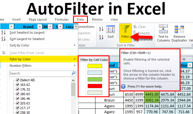
There are a few ways to turn on the filter functionality. The most common method is to select a cell within your data and then go to the Data tab and click the large Filter icon.
Let's watch a video that demonstrates how to enable filters and perform the most basic filtering operation: selecting specific values from a list.
This video from Kevin Stratvert provides a clear, step-by-step guide to using Excel's filter functionality.
First, watch the section on enabling filters. The video shows two methods: using the Filter button and converting your data to an Excel Table (a topic we will cover in detail later). For now, focus on the Filter button method. Next, watch the segment on basic text filtering. Pay attention to how you can: Click the filter arrow in a column header. Deselect "(Select All)" to clear the current selection. Check the boxes next to the specific values you want to see. Use the search box to quickly find the items you're looking for.
When you apply a filter, Excel doesn't delete the other rows; it simply hides them. You can tell a filter is active because the row numbers on the left will turn blue, and the icon in the column header changes from a simple dropdown arrow to a filter symbol.

Filtering with Conditions: Text, Numbers, and Dates
Simply selecting values from a list is useful, but the real power of filtering comes from applying specific conditions. Excel is smart enough to provide different conditional filters depending on whether the column contains text, numbers, or dates.
Text Filters
Instead of just selecting "New York" and "New Jersey," you could ask Excel to show all states that "Begin with 'New'" or "Contain 'land'". This is particularly useful for cleaning messy data or working with large, complex datasets.
Number Filters
When dealing with financial data, you'll frequently use number filters. You can instantly find all sales "Greater than $10,000," identify underperforming stores by filtering for profits "Less than or equal to $0," or even isolate the "Top 10 Items" by revenue.
Date Filters
Excel offers a fantastic range of dynamic date filters. You can filter for records from "Last Year," "This Quarter," or "Next Week" with a single click. You can also specify custom date ranges, such as "all activity between April 1st and June 30th."
The following video segments demonstrate these powerful conditional filters.
Continuing with Kevin Stratvert's video, let's explore these context-specific filters.
Please watch these three segments: Text Filters: from this section. Number Filters: from this part. Date Filters: from this final segment. For each type, notice the sub-menu that appears (e.g., Text Filters, Number Filters) and the variety of logical conditions available.
Advanced Techniques: Wildcards and Formatting
Two other powerful filtering methods can significantly speed up your work.
1. Filtering by Color:
If you or a client use cell colors to flag items—for instance, highlighting rows that need review in yellow—you can filter your data to show only the cells of a specific color. This also works with font colors and colors applied via conditional formatting.
Let's see a quick demonstration of filtering by color.
Watch the segment from this video on how to isolate rows based on their background color.
2. Using Wildcards in Text Filters:
Sometimes you need to find text that follows a certain pattern. Wildcards are special characters that can stand in for other characters. The two most common are:
*(asterisk): Represents any number of characters. For example, filtering for*shirtwould find "T-shirt", "shirt", and "blue shirt".?(question mark): Represents a single character. For example,gr?ywould find both "gray" and "grey".
Wildcards are extremely useful when dealing with inconsistent data entry.
Excel Filter Basics (for quick data analysis)
This video from Leila Gharani offers a great explanation of using wildcards in the filter's search box.
Watch from this section. Notice how she uses the asterisk (*) to find all products that contain the word "shirt", regardless of what comes before or after it.
Combining and Clearing Filters
Filters are additive. You can apply a filter to one column, and then apply another filter to a different column to further narrow down your results. For example, you could first filter the Region column to show only "North," and then filter the Sales column to show values "Greater than $500." The result would be only the sales over $500 that occurred in the North region.
Once you're done, you'll need to remove the filters to see all your data again. You can clear a filter from a single column or clear all filters on the worksheet at once.
This article from Excel Practice Online provides a concise written guide to clearing and combining filters.
First, read the two methods for returning to the original table under the heading "How do I go back?". Then, read the section that demonstrates combining filters for date and price, starting from "Using the Filter tool". This reinforces the additive nature of filters.
Time to Practice
Theory is one thing, but muscle memory is built by doing. The resource we just looked at provides a practice file. I strongly encourage you to download it and apply the techniques we've discussed.
This is your opportunity for hands-on practice.
In the article, find the section titled "Practice Filter tool" and click the link to download the exercise file. Once you have the file open, try to answer the following questions using filters: Show only the sales for "Laptops" and "Printers". Find all sales made by "John" that were greater than $400. Display all records from February 2020. Clear all filters.
Conclusion
You've now learned how to move beyond simply organizing data to actively interrogating it. Filtering is a daily-use skill for anyone who works with data in Excel.
Here are your key takeaways:
- AutoFilter hides rows that don't match your criteria, allowing you to focus on a subset of data.
- Activate filters using the
Filterbutton on theDatatab. - You can perform basic filtering by selecting values from the checklist or using the search box.
- Use conditional filters for text, numbers, and dates to apply specific criteria (e.g.,
Contains,Greater Than,This Month). - You can also filter by cell or font color, which is useful for visually tagged data.
- Filters are additive: you can apply them to multiple columns to progressively narrow your results.
- You can clear a single filter or all filters at once to return to your full dataset.
In our next lesson, we will explore Advanced Filtering. While AutoFilter is perfect for most day-to-day tasks, Advanced Filter allows you to build a separate criteria range on your worksheet to handle even more complex data extraction scenarios, such as queries involving intricate OR conditions across multiple columns.