Introduction
In our previous lesson, we explored sparklines, learning how to embed compact, word-sized graphics directly into cells for quick trend analysis. This is great for high-density dashboards. Now, we'll tackle a different, but equally important, challenge for professional report building: creating standard charts that stay current as your data grows.
This lesson focuses on creating dynamic charts—charts that automatically update when you add new data. As a freelancer, you'll build many reports for clients that track data over time (e.g., weekly sales, monthly expenses, daily web traffic). Manually adjusting chart ranges every time new data comes in is tedious, inefficient, and a common source of errors. Mastering dynamic charts will allow you to build "set it and forget it" reports that are robust and low-maintenance, a key value proposition for your clients.
To achieve this, we will leverage Excel Tables, a feature you were introduced to in Module 4. By the end of this lesson, you will be able to use Excel Tables to build charts that expand automatically, saving you time and ensuring your visualizations are always up-to-date.
1. The Problem: Static Charts and Manual Updates
By default, when you create a chart in Excel, it is linked to a fixed, or static, range of cells. If you add new data just below this range, the chart will not see it. You would have to manually edit the chart's source data to include the new rows. Let's see this problem in action.
The video "Excel Tables Tutorial" by the "Learn Google Sheets & Excel Spreadsheets" channel provides a perfect demonstration of this limitation, not with charts, but with formulas. The principle is exactly the same.
Excel Tables Tutorial - Dynamic Expandable Range
This video starts by clearly showing the problem that Excel Tables are designed to solve.
Watch the first couple of minutes, from the beginning to the end of the problem demonstration. Notice how adding a new number at the bottom of the list doesn't update the SUM or AVERAGE formulas. A chart based on the same static range would behave in exactly the same way—it would ignore the new data.
This is the core issue we need to solve. Imagine a client's weekly sales report. If you have to manually update every chart each Monday, you're wasting valuable time and introducing the risk of forgetting to update one, leading to an inaccurate report. We need a better way.
2. The Solution: Using Excel Tables as a Dynamic Source
The solution is to stop using static ranges and start using Excel Tables. As you may recall from Module 4, an Excel Table is not just a block of formatted cells; it's a special object that understands its own boundaries. Its most powerful feature for our purpose is that it automatically expands to include new data added in adjacent rows or columns.
When a chart uses an Excel Table as its source, it doesn't point to a static range like A1:B10. Instead, it points to the table itself. Therefore, when the table expands, the chart's source data expands with it, automatically.
Let's watch a quick demonstration of creating a table and seeing how it expands.
7 Reasons Why you Should use Excel Tables
The "7 Reasons Why you Should use Excel Tables" video gives a great, quick overview of how to create a table and its auto-expansion feature.
First, watch the segment on creating a table. You'll see a few different methods, including the Ctrl+T shortcut. Then, observe how the table expands when a new row or column is typed next to it. This is the magic that makes our charts dynamic.
By basing our charts on this auto-expanding object, we ensure they always reflect the complete dataset.
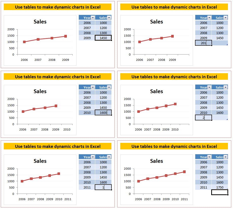
3. Hands-On: Building Your First Dynamic Chart
Now, let's put this into practice. Your preference for hands-on learning is key here, so we'll walk through the process step-by-step.
We'll start with a simple dataset.
- Open a new Excel worksheet.
- Enter the following data starting in cell
A1:
| Month | Sales |
|---|---|
| Jan | 1500 |
| Feb | 1800 |
| Mar | 1650 |
| Apr | 2100 |
Step 1: Convert the Range to an Excel Table
First, we need to turn this simple range into a proper Excel Table.
- Click any cell inside your data (e.g.,
A2). - Press Ctrl + T on your keyboard.
- The Create Table dialog box will appear. Excel correctly identifies the range
=$A$1:$B$5. - Ensure the box for My table has headers is checked.
- Click OK.
Your data is now a formatted Excel Table.
Step 2: Create a Chart from the Table
Now, let's create our chart.
- Click anywhere inside your new table.
- Go to the Insert tab on the ribbon.
- In the Charts group, click on Insert Column or Bar Chart and select the first 2-D Column chart.
Excel will insert a column chart based on your table data.
Step 3: Test the Dynamic Behavior
This is the moment of truth. Let's add new data for May.
- Click on cell
A6(the cell directly below "Apr"). - Type "May" and press Tab.
- Notice how the table's border and formatting automatically expand to include this new row.
- In cell
B6, type a new sales value, for example,2300, and press Enter.
Look at your chart. It has automatically updated to include the bar for May! You did not have to touch the chart at all. This is the power of dynamic charts.
For a detailed written guide that you can refer back to, the following article from Excel University is excellent.
How to Make an Excel Dynamic Chart & Keep Updates ...
This article provides a clear, concise walkthrough of the exact process we just followed. It's a great resource to bookmark for future reference.
Read the section titled Creating a Dynamic Chart Using a Table. It reinforces the steps and the "auto-expand" behavior you just experienced.
4. Important Considerations
The method of using Excel Tables is by far the most straightforward and recommended way to create dynamic charts. The TrumpExcel article provides another excellent walkthrough and highlights a key detail about deleting data.
How to Create a Dynamic Chart Range in Excel
This article reinforces the table-based method and adds an important note on what happens when you delete data.
Please read the section Using Excel Table. Pay special attention to the note about deleting data. While adding data automatically expands the chart, deleting rows might leave empty space. The article shows how to manually drag the small blue handle in the bottom-right corner of the table to resize it if needed.
It's also worth knowing that a more complex, formula-based method exists using functions like OFFSET and COUNTA. The articles from both TrumpExcel and Excel University describe this technique. You don't need to learn it now, as Tables are superior for this task, but it's good to be aware that it's possible, especially if you ever work with very old versions of Excel that don't support Tables.
Conclusion
You have now learned a fundamental skill for building professional, automated reports. By basing your charts on Excel Tables instead of static ranges, you create dynamic visualizations that automatically adapt to new data. This not only saves you significant time and effort but also reduces the risk of human error, resulting in more reliable and professional client deliverables.
Key Takeaways:
- Standard Excel charts are static; they are tied to a fixed data range and do not update when new rows are added outside that range.
- An Excel Table is a dynamic object that automatically expands to include new, adjacent data.
- By creating a chart from an Excel Table, the chart becomes dynamic, automatically updating its data source as the table grows.
- The process is simple: convert your data range to a Table (Ctrl + T), then insert a chart based on that table.
In our next lesson, we will build on this foundation. Now that we have charts that update automatically, we will learn how to add interactive controls like Slicers and Timelines. This will allow you and your clients to filter your dynamic charts with the click of a button, bringing us one step closer to building fully interactive dashboards.