Mastering Data Visualization: Creating and Customizing Charts

Introduction

In our last lesson, we mastered the essential techniques for keeping PivotTable reports current and accurate, ensuring our data analysis is always based on the latest information. Now that we can trust our summarized data, it's time to bring it to life. A table of numbers can hold valuable insights, but a well-designed chart can tell a story, reveal a trend, or highlight a relationship in a single glance.

This lesson marks our entry into the world of data visualization. We will focus on creating and customizing the most fundamental and widely used chart types in Excel: bar, column, line, and scatter charts. For you as a future freelance analyst, mastering visualization is not just about making data look pretty; it's about communicating your findings clearly and persuasively to clients. This is the first step toward building the professional, interactive dashboards that are a cornerstone of data analysis and reporting.

1. Why Visualize? Choosing the Right Chart for the Job

Before we start creating charts, it's crucial to understand their purpose. Data visualization is the art and science of representing data graphically to make it easier to understand. A good chart can help you and your audience quickly identify trends, patterns, and outliers that might be hidden in a spreadsheet.

To represent data effectively, you must choose a chart type that matches the story you want to tell. While Excel offers a vast library of charts, a few workhorses cover most analytical needs.

How to Make Charts and Graphs in Excel

This article from Smartsheet provides an excellent overview of the primary chart types and their uses.

Focus on the descriptions for Column and Bar Charts, Pie Charts, Line Charts, and Scatter Charts. As you read, think about the kind of data you would use for each.

To summarize the key ideas from the reading:

To Show...	Use a...	Because...
Comparison between different categories.	Column Chart or Bar Chart	It's easy to compare the lengths of the bars representing each category's value.
Trends over a period of time.	Line Chart	It connects data points, clearly showing increases, decreases, or volatility over time.
The relationship between two numeric variables.	Scatter Chart	It plots pairs of values, revealing correlations (or a lack thereof) between them.
Proportion, or parts of a whole.	Pie Chart	It represents a total amount as a "pie," with each slice showing the percentage contribution of its category.

Understanding these fundamental uses is the first step toward creating meaningful visualizations instead of just decorative ones.

2. Creating Your First Chart

The process of creating a chart in Excel is straightforward. It generally involves just three steps:

Select your data: Highlight the cells containing the data you want to visualize, including the headers for your rows and columns.
Insert the chart: Go to the Insert tab on the ribbon.
Choose a chart type: Select the chart that best tells your data's story.

Let's watch a demonstration of this core workflow.

Excel Charts and Graphs Tutorial

The video "Excel Charts and Graphs Tutorial" by Kevin Stratvert provides a clear, beginner-friendly introduction to inserting charts.

First, watch from the initial segment to see how to select data and use Excel's "Recommended Charts" feature. This is a great starting point when you're not sure which chart to use. Then, watch the section on shortcuts from using Alt+F1. The Alt + F1 shortcut instantly creates a default chart on the current worksheet and is a fantastic productivity booster.

Now that you've seen the basic process, let's get some hands-on practice with the specific chart types mentioned in our learning goal.

3. A Practical Guide to Key Chart Types

For the following exercises, we will use a sample dataset. The DataCamp tutorial "Visualizing Data in Excel" provides a simple sales dataset that is perfect for this.

Visualizing Data in Excel

This article includes an easy-to-use dataset.

Find the table under the Example Dataset heading and copy-paste it into a new Excel workbook. This will be your practice file for the rest of the lesson.

Column and Line Charts

Column charts are excellent for comparing sales across different product categories, while line charts are ideal for tracking sales performance over time.

Visualizing Data in Excel

This section provides clear, step-by-step instructions for creating these fundamental charts.

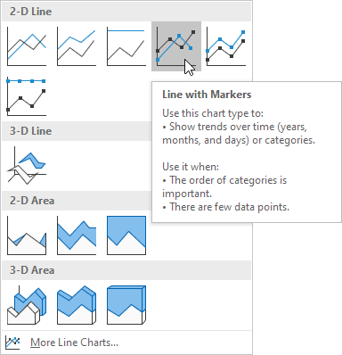
Follow the instructions under the headings Excel column charts and Excel line charts using the sample data you just copied. For the line chart, you will be creating a "Line with Markers" chart, as shown in the image below.

The "Line with Markers" option is often preferred as it makes the individual data points for each month clearly visible.

Scatter Charts

Scatter charts help us investigate the relationship between two different variables. For example, does advertising spending correlate with items sold? Or in our sample data, is there a relationship between the number of TVs sold and Laptops sold each month?

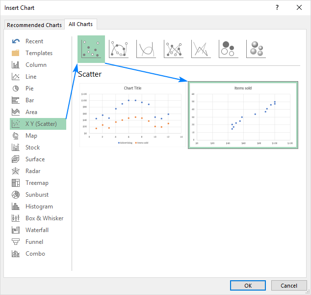
Let's create one to see if there's a connection between TV and Mobile Phone sales.

Select the data range for Month, TVs, and Mobile Phones (e.g., A1:C13 in the sample data).
Go to the Insert tab, click the Scatter (X, Y) chart icon, and choose the simple Scatter option.

Excel will plot one series against the other. Each point on the chart represents a month, showing the number of TVs sold on one axis and Mobile Phones on the other. This visual can quickly tell you if months with high TV sales also tend to have high Mobile Phone sales.

4. Customizing Charts for Clarity and Impact

Creating a chart is just the beginning. A default chart is functional, but a customized chart is professional and communicates effectively. As a freelancer, the quality of your chart formatting directly reflects the quality of your work.

Excel provides a wealth of customization options through three main access points when a chart is selected:

The Chart Design and Format tabs that appear on the ribbon.
The plus sign (+) icon that appears to the right of the chart for adding or removing chart elements.
The Format Pane, which you can open by double-clicking any chart element or by selecting an element and pressing Ctrl + 1.

Let's see how these are used to polish a chart.

Excel Charts & Graphs: Learn the Basics for a Quick Start

The video "Excel Charts & Graphs" by Leila Gharani offers a fantastic, concise tour of the core formatting tools.

Watch the segment from customizing elements. Pay close attention to how she uses the plus sign icon to add elements like data labels and the Format Pane (Ctrl+1) to access detailed options. The Format Pane is your command center for fine-tuning every aspect of your chart.

Based on the video, here are the essential elements you should learn to customize:

Chart Title: Always give your chart a clear, descriptive title. You can also link the title to a cell for dynamic updates, as shown in the first video by Kevin Stratvert at 08:19.
Axis Titles: Label your X and Y axes so your audience knows exactly what they are looking at (e.g., "Month", "Units Sold").
Legend: The legend explains what each data series (e.g., each colored line or bar) represents. Position it where it's clear but not intrusive.
Data Labels: Sometimes it's helpful to show the exact value of a data point directly on the chart. Use them sparingly to avoid clutter.
Gridlines: These can help guide the reader's eye from an axis to a data point, but overly heavy gridlines can be distracting.
Trendline: For line and scatter charts, adding a trendline can visually represent the overall direction or pattern in the data.

Take some time now to practice. Using the column chart you created earlier, try to perform the following customizations:

Change the chart title to "2022 Electronics Sales".
Add a vertical axis title and name it "Units Sold".
Move the legend to the top of the chart.
Experiment with different Chart Styles from the Chart Design tab.
Change the color scheme using the Change Colors button.

Conclusion

In this lesson, you've taken your first and most important steps into data visualization in Excel. You've learned not just how to create charts, but more importantly, why and when to use specific types to effectively communicate insights.

Key Takeaways:

Choose your chart type based on your goal: bar/column charts for comparison, line charts for trends over time, and scatter charts for relationships.
The basic workflow is to select data, insert the chart, and then customize it.
Effective customization is key to professional reporting. Master the use of the Chart Design/Format tabs and the Format Pane (Ctrl+1) to control titles, axes, legends, and colors.
A well-designed chart tells a clear story, turning raw data into actionable insight for you and your clients.

In our next lesson, we will bridge the gap between our last two topics. You'll learn how to create PivotCharts, which are dynamic charts built directly on top of a PivotTable, allowing for powerful, interactive data visualization.

Recommended resources