Welcome back! In our previous lesson, we constructed a complete project tracker, combining your skills in formulas, conditional formatting, and data structures to build a valuable, client-ready tool. That exercise was about managing tasks and timelines. Now, we'll apply a similar tool-building mindset to a different, but equally important, domain: financial analysis.
This lesson focuses on creating a sophisticated financial calculator. Specifically, you will learn how to build a dynamic mortgage calculator that not only determines monthly payments but also models the impact of extra payments and allows for scenario comparison. This is a common and highly practical tool that showcases a developer's ability to translate complex financial concepts into a user-friendly Excel interface, building directly on the financial modeling functions you learned in Module 8.
By the end of this lesson, you will be able to construct a professional financial calculator from scratch, integrating key financial functions with a well-designed user interface.
The Anatomy of a Financial Calculator
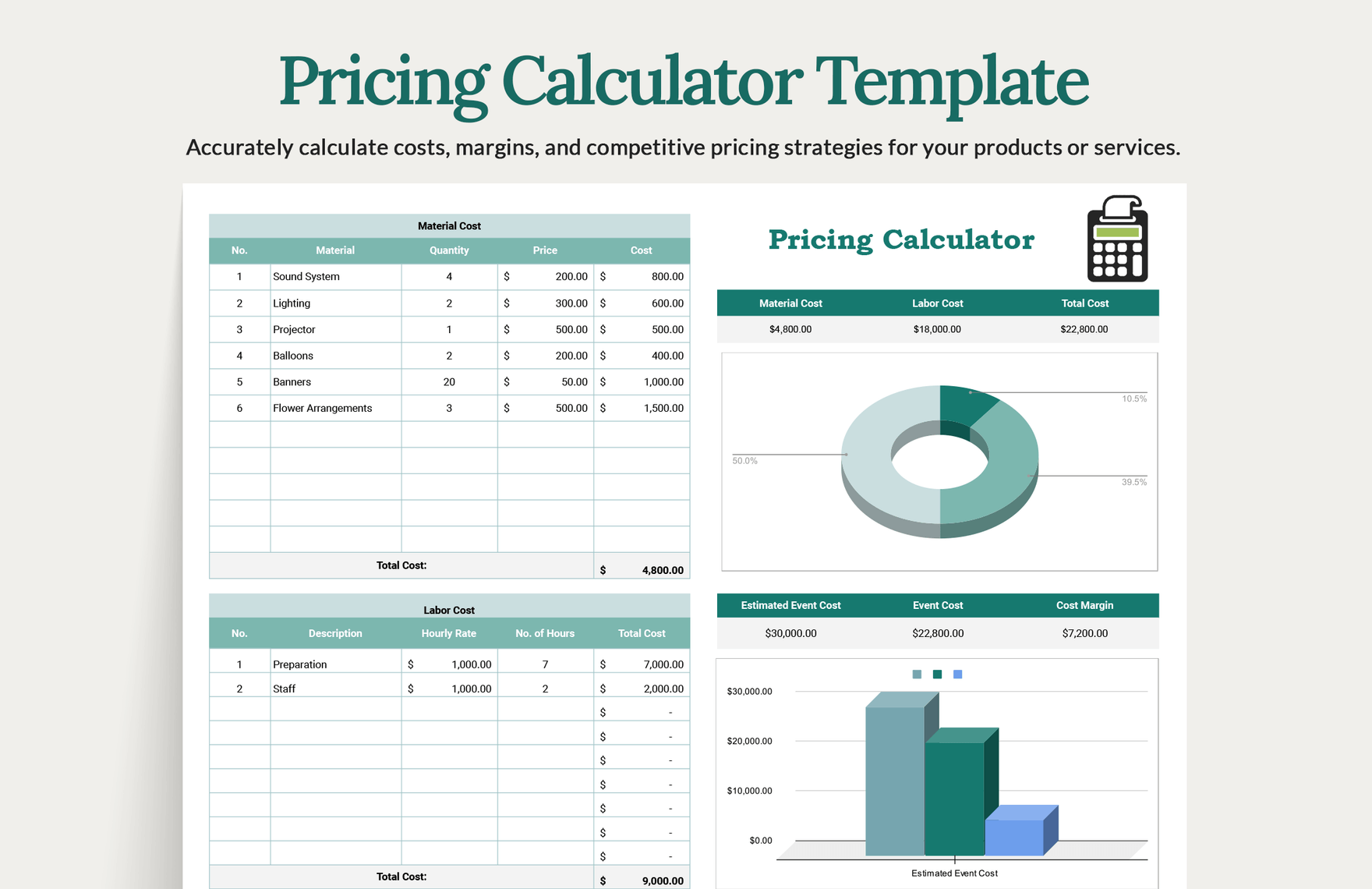
Before we start building, let's consider the structure. A professional tool, whether for project management or finance, should be clean, intuitive, and clearly separate user inputs from the calculated outputs. This makes the tool easy to use and hard to break.
A mortgage calculator is an excellent example. At its core, it takes a few key inputs—loan amount, interest rate, and term—and performs a series of calculations to produce an amortization schedule and summary analysis.
Step 1: Calculating the Core Monthly Payment
The foundation of any loan calculator is the periodic payment. Excel's suite of time value of money functions makes this straightforward. The primary function we'll use is PMT.
The PMT function calculates the payment for a loan based on constant payments and a constant interest rate. Its syntax is:
=PMT(rate, nper, pv, [fv], [type])
rate: The interest rate for the period. For a mortgage with an annual rate, you'll divide this by 12.nper: The total number of payment periods. For a 30-year mortgage with monthly payments, this is 30 * 12.pv: The present value, or the total amount that a series of future payments is worth now. This is the loan principal.
The following video provides a clear, practical demonstration of setting up the initial loan parameters and using the PMT function.
Excel Mortgage Calculator | Extra Payments
This video from HowToAnalyst starts by setting up the basic loan information and calculating the monthly payment.
Watch the first part of the video, from the beginning to the PMT calculation. Pay attention to how the annual figures (APR and years) are converted to monthly periods for the rate and nper arguments. Notice that Excel returns a negative value, which the presenter corrects by adding a negative sign to the pv argument or the whole formula; this is standard practice as the loan represents a cash outflow to the lender.
Step 2: Building the Amortization Schedule
With the monthly payment calculated, the next step is to show how each payment is broken down into interest and principal over the life of the loan. This is the amortization schedule. It's the engine of our calculator.
The schedule tracks the following for each period:
- Beginning Balance: The outstanding loan amount at the start of the month.
- Interest: The portion of the payment that covers the interest accrued for that month. Calculated as
Beginning Balance * monthly rate. - Principal: The portion of the payment that reduces the loan balance. Calculated as
Payment - Interest. - Extra Payment: A crucial field for our dynamic calculator, allowing the user to input additional principal payments.
- Ending Balance: The new loan balance after all payments. Calculated as
Beginning Balance - Principal - Extra Payment.
Let's continue with the same video to see how to build this table.
Excel Mortgage Calculator | Extra Payments
The video now guides you through constructing the full amortization table, row by row.
Watch the section from building the columns. This is the most critical part of building the calculator's logic. Observe how: The SEQUENCE function is used to quickly generate the period numbers. The beginning balance of the first period is the total loan amount. For all subsequent periods, the beginning balance is simply the ending balance of the previous period. This iterative, row-by-row calculation is fundamental. Formulas for interest and principal are created and then copied down the entire table. Notice the use of absolute references (F4) to lock the cells containing the APR and total payment.
This "traditional" row-by-row approach is powerful because it allows for dynamic changes, like extra payments, that affect all subsequent rows. While there are more advanced single-formula methods, this traditional build is easier to understand, debug, and is a core skill for any Excel developer.
Mortgage payment schedule - Excel formula
The Exceljet article provides an excellent written breakdown of this traditional approach, reinforcing the concepts from the video.
Please read the section on the Traditional formula solution. This will give you a clear, step-by-step text reference for the formulas used in the first row versus subsequent rows and explains why they are different. It also introduces the useful practice of creating named ranges (loan, rate, etc.) to make your formulas more readable, a technique you learned in Module 2.
Step 3: Creating a User-Friendly Summary
An amortization table with 360 rows is not a user-friendly output. To make our calculator a true "tool," we need to add a summary section that clearly displays the most important results. What does the user want to know?
- How much interest will I save if I make extra payments?
- How much sooner will I pay off my loan?
To answer these questions, we need to calculate summary metrics that compare the loan with extra payments to the loan without them. The video you've been watching demonstrates how to calculate these valuable outputs.
Excel Mortgage Calculator | Extra Payments
This final section of the video focuses on building the summary dashboard that calculates interest and month savings.
Watch the segment from calculating savings. This part introduces some advanced formula usage: Original Interest (IPMT): The IPMT function is used to calculate the interest portion for a given period of a standard loan. By summing this for all periods, we get a baseline for total interest without any prepayments. Interest Saved: This is simply the difference between the baseline interest and the sum of the interest column from our dynamic schedule. Months Saved: A clever XLOOKUP is used to find the first period where the ending balance drops below zero, indicating the loan is paid off. The difference between the original term (360 months) and this payoff period gives the months saved.
Step 4: Adding Interactivity with Scenarios
To elevate your tool from a calculator to a decision-making dashboard, you can add scenario analysis. This allows a user to quickly toggle between different assumptions (e.g., a "Base Case" with no extra payments vs. an "Aggressive Case" with a $500 extra monthly payment) and see the impact instantly.
The CHOOSE function is perfect for this. It returns a value from a list of arguments based on an index number.
For example, imagine you have a cell (let's say F1) where the user enters 1 for the Base Case and 2 for the Aggressive Case. You have two other cells with the extra payment amounts: F2 with 0 and F3 with 500.
In your amortization schedule's "Extra Payment" column, instead of referencing a single cell, you could use:=CHOOSE($F$1, $F$2, $F$3)
If the user enters 1 in F1, the formula returns the value from F2 (0). If they enter 2, it returns the value from F3 (500). The entire amortization schedule and summary section will update instantly.
The following video, while demonstrating a full financial model, has a brilliant section that perfectly illustrates this technique.
Build a Dynamic Financial Model in Just 15 Minutes
This video by Kenji Explains shows how to make a financial model dynamic using scenario analysis with the CHOOSE function.
Watch the section focused on making the model dynamic. Focus on the core concept: Multiple sets of assumptions are created. A single "Live" assumption table is created that will feed the model. The CHOOSE function is used in the "Live" table to pull data from the different assumption sets based on a single scenario selector cell. You can apply this exact logic to your mortgage calculator's "Extra Payment" input to create a powerful scenario toggle.
Conclusion
In this lesson, you have moved from a blank sheet to a powerful, user-friendly financial tool. You've seen how to combine financial functions with a well-structured layout and dynamic formulas to create a calculator that not only provides answers but also helps users make informed decisions.
Key Takeaways:
- A professional calculator separates inputs, calculations, and outputs.
- The
PMTfunction is the starting point for calculating a loan's periodic payment. - An amortization schedule is built using iterative, row-by-row formulas where each period depends on the previous one. This structure is key to modeling dynamic changes like extra payments.
- A summary dashboard is essential for a user-friendly interface, translating the raw data of the schedule into meaningful insights like "Interest Saved" and "Months Saved."
- The
CHOOSEfunction is a powerful way to enable scenario analysis, allowing users to toggle between different sets of assumptions and immediately see the results.
In our next lesson, we will build upon the tool you've designed today. We'll explore how to make it "bulletproof" by applying advanced data validation (like creating a dropdown menu for the scenario selection) and cell protection to prevent users from accidentally breaking your intricate formulas.