Welcome to the final module of your course! Having explored a wide array of Excel's capabilities, from data transformation in Power Query to automation with VBA, we now begin to synthesize these skills to create complete, client-ready solutions. In the last lesson, you learned how to programmatically send emails from Excel, a powerful way to distribute reports and communicate updates. Now, we'll shift our focus back to building the sophisticated content that warrants such automation.
This lesson addresses the first major project of this module: designing and building a dynamic project tracker. This is a common and highly valuable tool for freelance Excel developers to create. You will learn how to structure project data, calculate key metrics like overdue tasks, and create compelling visualizations—including a full Gantt chart—using the formulas and conditional formatting skills you've acquired.
By the end of this lesson, you will be able to construct a professional and interactive project management template from the ground up, integrating multiple techniques into a single, cohesive tool.
Designing the Core: The Data and Dashboard
Every great project tracker starts with a well-structured data table. The foundation of a dynamic tracker is the Excel Table, a feature you first encountered in Module 4. It ensures that all our formulas and charts will update automatically as new tasks are added.
From this data foundation, we can build a high-level dashboard that provides an at-a-glance summary of the project's health. This includes key performance indicators (KPIs) like the number of completed, in-progress, or overdue tasks.

The following video provides an excellent walkthrough of building a comprehensive task management dashboard. It's a fantastic practical application of many skills you've learned.
Make a Dynamic Task Management Tracker in Excel!
This video by Kenji Explains demonstrates how to build a dynamic dashboard from a task list, integrating formulas, charts, and conditional formatting.
Please watch the video, paying close attention to these key stages of development: Data Setup (watch this part): Notice the immediate conversion of data to an Excel Table (Ctrl+T). This is a best practice. Dynamic Calculations (watch this part): See how a formula using AND and TODAY is used to create a "True/False" flag for overdue tasks. This is a core concept for dynamic trackers. Ensuring Data Integrity (watch this part): The use of Data Validation to create dropdown lists for statuses prevents user error and ensures your formulas work correctly. Building KPIs (watch this part): Pay attention to the clever use of the COUNTIF function to calculate the number of tasks for each status, and how these values are linked to text boxes on the dashboard for a clean presentation. Visualizing Workload (watch this part): Observe how simple bar charts are created to show task distribution by owner and team, then formatted and placed on the dashboard. Visual Task Status (watch this part): This section demonstrates applying conditional formatting to automatically color-code the status column, making the raw data much easier to interpret.
Visualizing the Timeline: The Gantt Chart
While a dashboard gives a great summary, clients often want to see a project timeline, known as a Gantt chart. This visual shows the start and end dates of tasks and their relationships over time. There are two primary ways to create a Gantt chart in Excel.
Method 1: The Classic Stacked Bar Chart
The traditional method uses a stacked bar chart. You create a chart with two data series: the "Start Date" and the "Duration". Then, you make the "Start Date" series invisible by setting its fill to 'No Fill'. The remaining visible bars represent the task durations, positioned correctly along the timeline.
The following article explains this process step-by-step.
How to Build a Dynamic Gantt Chart in Excel
This article from Office Productivity Training provides a clear, structured guide to the stacked bar chart method and introduces the critical concept of task dependencies.
Please read through the first four steps of the article to understand the classic approach: Step 1 and the start of Step 2: Focus on the recommended table structure. Crucially, this introduces the Predecessor column, which is used to create task dependencies. The formula provided is a brilliant synthesis of IF, WORKDAY, INDEX, and structured references: =IF([@Predecessor]<>"", WORKDAY(INDEX([End Date],[@Predecessor]),1), [@[Manual Start Date]]) This formula checks if a predecessor task exists. If it does, the current task's start date is set to the first working day after the predecessor ends. Otherwise, it uses a manually entered start date. Step 3: This shows you how to add the Start Date and Duration data to the chart. Step 4: This covers the key formatting tricks: hiding the Start Date series and reversing the task order on the vertical axis so it matches your data table.
Method 2: The Advanced Conditional Formatting Gantt Chart
A more modern and visually integrated approach is to build the Gantt chart directly in the worksheet grid using conditional formatting. This technique requires more complex formulas but results in a highly polished and professional-looking tracker that looks like it was made in dedicated project management software like Microsoft Project.
Given your goal of becoming an expert freelancer, mastering this advanced technique can set your work apart.
How to Make the BEST Gantt Chart in Excel (looks like Microsoft Project!)
This video by David McLachlan is a masterclass in building a top-tier Gantt chart using conditional formatting.
This is a detailed video, so focus on these key implementation sections: Creating the Calendar (watch this part): Understand how the dynamic date headers for days, months, and years are created. This calendar is the backbone of the chart. Calculating Work Days (watch this part): The NETWORKDAYS function is used here to calculate the duration, automatically excluding weekends. Building the Gantt Bars (watch this part): This is the core of the technique. Pay close attention to how multiple conditional formatting rules with complex AND formulas are layered to create the visual bars. A new rule is created for each visual element: the main task bar, the progress within the bar, the indicator for completed tasks, and the highlight for blocked tasks. Improving Usability (watch this part): A simple but crucial final touch: using Freeze Panes to keep the task names and calendar headers visible while scrolling.
Highlighting Overdue Tasks: A Critical Feature
No project tracker is complete without a clear, unmissable indicator for tasks that are falling behind. This is a perfect use case for conditional formatting with a formula. We want to highlight any task that is not yet "Done" and whose due date is in the past.
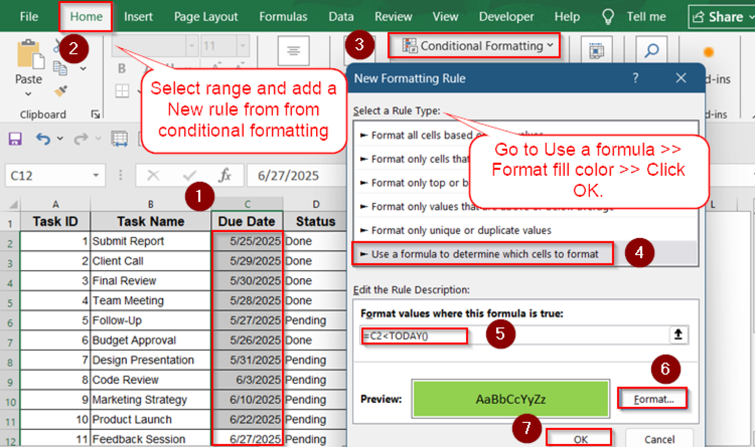
The formula to achieve this is a simple combination of AND and TODAY. For a table where the due date is in column C and the status is in column D, the formula to highlight the entire row would be:
=AND($C2<TODAY(), $D2<>"Done")
Let's break this down:
$C2<TODAY(): Checks if the due date in column C is before today's date. The dollar sign$locks the column, allowing the format to be applied across the row.$D2<>"Done": Checks if the status in column D is anything other than "Done".AND(...): Requires both conditions to be true for the formatting to be applied.
Conditional Formatting to Highlight Overdue Dates in Excel
This article provides a concise guide to this essential formatting rule.
Review the sections on "Focus on Overdue Tasks with Specific Status" and "Highlight Entire Row for Overdue Tasks". Note the use of the dollar sign $ to lock columns when applying a format to a whole row.
Conclusion
In this lesson, you've learned how to design and build a sophisticated, dynamic project tracker—a cornerstone project for any Excel developer. You have combined your knowledge of Excel Tables, advanced formulas, and conditional formatting to create a tool that is both functional and visually impressive.
Key Takeaways:
- A dynamic project tracker is built on an Excel Table to ensure formulas and charts update automatically.
- A dashboard view with KPIs (using
COUNTIF) and summary charts provides a high-level project overview. - Data Validation is crucial for maintaining data integrity, especially for status fields.
- Gantt charts can be created using a classic stacked bar chart method or a more advanced technique using layered conditional formatting rules.
- Formulas combining
AND,TODAY, and cell references are essential for creating dynamic visual cues, such as highlighting overdue tasks. - Task dependencies can be modeled using a combination of
IF,WORKDAY, andINDEXfunctions, creating a truly interconnected project plan.
In our next lesson, we will continue our journey of building professional tools by constructing a financial calculator. This will shift our focus to applying your financial modeling and user interface skills to create another valuable, client-ready asset.