Creating PivotTables from Data

1. From Raw Data to Insight: What is a PivotTable?

Imagine you have a spreadsheet with thousands of rows of sales data. Your manager asks, "What were the total sales for each region?" or "How many units of each product did we sell?" You could try to answer this with formulas like SUMIF, but as the questions get more complex, the formulas become unwieldy.

This is precisely the problem PivotTables solve. They allow you to take a large, flat table of data and "pivot" it into a summarized report. You can dynamically rearrange the report by dragging and dropping fields to answer different questions in seconds.

To understand the difference between raw data and a PivotTable summary, let's watch a brief introductory clip.

2. Preparing Your Data for Success

Before you create a PivotTable, you must ensure your data is well-structured. This means:

• Your data should be in a tabular format, with each column having a unique header in the first row.
• There should be no blank rows or columns within your dataset.

While you can create a PivotTable from a simple range of cells, it is a strong best practice to first convert your data into an Excel Table. As you may recall from Module 4, an Excel Table provides several advantages. For PivotTables, the most important benefit is that they are dynamic. If you add new rows of data to your source Table, your PivotTable will automatically include them the next time you refresh it.

Let's see how to quickly convert a data range into an Excel Table.

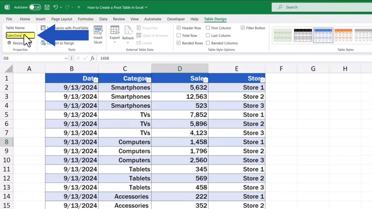
Once you've created a table, it's also good practice to give it a meaningful name. You can do this from the Table Design tab that appears when you select any cell within the table. Naming your table "SalesData" is much clearer than using the default "Table1".

3. Creating Your First PivotTable

With your data prepared in an Excel Table, you are ready to create the PivotTable itself. The process involves just a few clicks.

1. Click any single cell inside your Excel Table.
2. Go to the Insert tab on the ribbon.
3. Click PivotTable.

This will open the "Create PivotTable" dialog box. Because you started from within an Excel Table, Excel automatically populates the Table/Range field with your table's name. You then choose where to place the new PivotTable report: in a new worksheet (most common) or on an existing one.

This next video will walk you through this exact process.

4. Understanding the PivotTable Interface

After you click OK, Excel creates a new worksheet with a PivotTable placeholder on the left and a PivotTable Fields pane on the right. This pane is your control center for building the report. If you ever click outside the PivotTable area and the pane disappears, simply click back into the placeholder to make it reappear.

Let's break down what you're seeing.

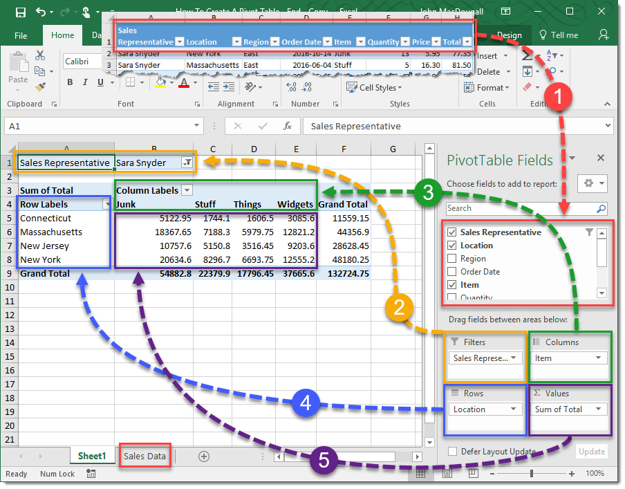
As shown in the image above, the PivotTable Fields pane has two main sections:

1. Field List: At the top is a list of all the column headers from your source data. Each of these is a "field" you can use to build your report.
2. Layout Areas: At the bottom are four boxes that represent the different parts of your report. You build the report by dragging fields from the list above into these boxes.
   • Rows: Fields placed here will become the row labels of your report. Each unique item in the field gets its own row.
   • Columns: Fields placed here become the column labels.
   • Values: This area is for the fields you want to calculate. It typically holds numeric data that will be summed, averaged, or counted.
   • Filters: Fields placed here allow you to apply a high-level filter to your entire report.

For today, we will focus on the two most fundamental areas: Rows and Values.

5. Building a Basic Summary Report

Now it's time to bring your PivotTable to life. Let's say we want to answer the question: "What are the total sales for each salesperson?"

To build this report, you simply:

1. Drag the Salesperson field from the Field List and drop it into the Rows area.
2. Drag the Sales Amount field and drop it into the Values area.

Instantly, the PivotTable on the left will update. It will list each unique salesperson in a separate row and show the sum of their sales next to them. You've just created a powerful summary report in seconds, with no formulas required.

Let's watch this in action.

6. Practice Makes Permanent

The best way to solidify your understanding is to build a PivotTable yourself. The following resource provides a downloadable workbook with practice problems.

Conclusion

In this lesson, you have taken the first crucial step into the world of PivotTables. You've learned that they are not as intimidating as they might seem and are incredibly powerful tools for turning raw data into meaningful summaries.

Key Takeaways:

• A PivotTable summarizes large datasets, allowing you to "pivot" the data to see different perspectives.
• Always start with clean, tabular data, and it is a best practice to convert your data into an Excel Table before creating a PivotTable.
• You create a PivotTable using the Insert > PivotTable command.
• The PivotTable Fields pane is your control center, where you build reports by dragging fields into the Rows, Columns, Values, and Filters areas.

You now have a solid foundation for creating a basic PivotTable. In our next lesson, we will build upon this by exploring the Values area in more detail. You'll learn how to change the summary calculation from a sum to a count, average, minimum, or maximum, and how to display values as percentages of a total.