Calculating Regression Metrics

Evaluating Regression Models: How Far Off Are We?

For regression, accuracy is not a useful concept. A prediction of 150.1 is not "wrong" if the true value is 150.0; it's just slightly off. We need metrics that quantify the magnitude of this error.

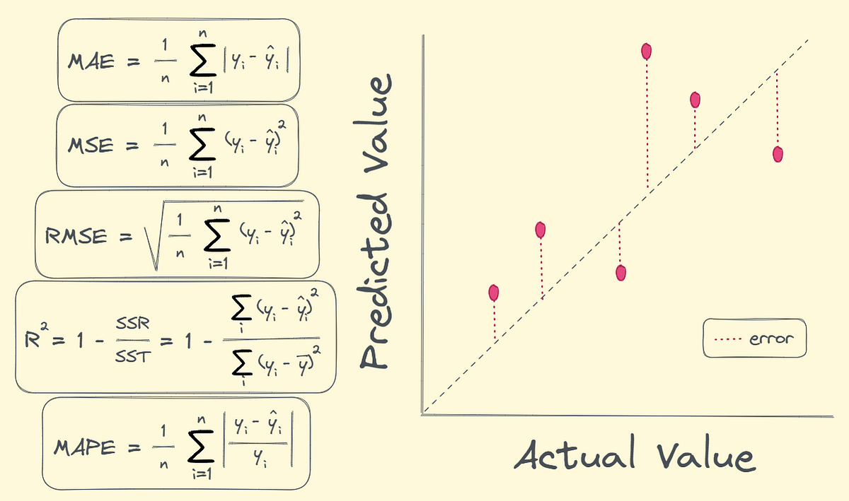
Let's dive into implementing the two most common regression metrics from scratch.

1. Mean Squared Error (MSE)

The Mean Squared Error is arguably the most common metric and loss function in regression. It measures the average of the squared differences between the actual values and the predicted values.

The formula is:
$\text{MSE}=\frac{1}{n}{\sum }_{i=1}^n(y_i-{\hat{y}}_i{)}^2$
Where:

• $n$ is the number of data points.
• $y_i$ is the actual (true) value for the $i$-th data point.
• ${\hat{y}}_i$ is the value predicted by the model for the $i$-th data point.

We square the error (y_i - \hat{y}_i) for two main reasons:

1. It makes all error values positive, so that negative errors don't cancel out positive ones.
2. It penalizes larger errors much more heavily than smaller ones. An error of 4 becomes 16, while an error of 2 only becomes 4.

Implementation from Scratch

Given your proficiency with Python and NumPy, we can implement this efficiently. The following video walks through the definition of MSE and implements it in a few ways.

Drawing from that logic, a clean, "from-scratch" implementation using NumPy is surprisingly simple. Your experience with NumPy's array operations will make this feel natural.

import numpy as np

def mean_squared_error(y_true, y_pred):
    """
    Calculates the Mean Squared Error from scratch using NumPy.
    
    Args:
        y_true (np.ndarray): Array of true target values.
        y_pred (np.ndarray): Array of predicted values.
        
    Returns:
        float: The calculated MSE.
    """
    # The difference between true and predicted values is the error.
    errors = y_true - y_pred
    
    # Square the errors.
    squared_errors = errors ** 2
    
    # Return the average of the squared errors.
    return np.mean(squared_errors)

# --- Example ---
y_true_example = np.array([3, -0.5, 2, 7])
y_pred_example = np.array([2.5, 0.0, 2, 8])

mse = mean_squared_error(y_true_example, y_pred_example)
print(f"MSE: {mse}") # Expected output: (0.5^2 + (-0.5)^2 + 0^2 + (-1)^2) / 4 = 0.375

Interpretation: The MSE is an absolute measure of error. A lower value is always better. However, its units are the square of the target's units (e.g., "dollars squared"), which can be hard to interpret. This is why we often use another metric for reporting: R-squared.

2. R-squared (R²) or Coefficient of Determination

While MSE gives us an absolute error value, R-squared provides a relative measure of how well the model performs compared to a naive baseline. This baseline model is one that simply predicts the mean of all true target values, regardless of the input features.

R-squared answers the question: "What proportion of the variance in the target variable is explained by our model?"

The formula looks like this:
$R^2=1-\frac{{\sum }_{i=1}^n(y_i-{\hat{y}}_i{)}^2}{{\sum }_{i=1}^n(y_i-\bar{y}{)}^2}=1-\frac{\text{Sum of Squared Residuals (SSR)}}{\text{Total Sum of Squares (SST)}}$
Where:

• The numerator, SSR, is the sum of our model's squared errors (what MSE is based on).
• The denominator, SST, is the sum of the squared errors of the naive "mean" model.
• $\bar{y}$ is the mean of the true values.

Implementation from Scratch

The following video provides an excellent walkthrough of programming the R-squared value from its core components.

Following the logic from the video and using vectorized NumPy operations, we can write a concise function.

def r_squared(y_true, y_pred):
    """
    Calculates the R-squared (coefficient of determination) from scratch.
    
    Args:
        y_true (np.ndarray): Array of true target values.
        y_pred (np.ndarray): Array of predicted values.
        
    Returns:
        float: The calculated R-squared value.
    """
    # Calculate the total sum of squares (SST).
    # This is the error of a model that just predicts the mean.
    sst = np.sum((y_true - np.mean(y_true)) ** 2)
    
    # Calculate the sum of squared residuals (SSR).
    # This is the error of our actual model.
    ssr = np.sum((y_true - y_pred) ** 2)
    
    # Calculate R-squared. Add a small epsilon to SST to prevent division by zero.
    r2 = 1 - (ssr / (sst + 1e-8))
    
    return r2

# --- Example using the same data ---
r2 = r_squared(y_true_example, y_pred_example)
print(f"R-squared: {r2}")

Interpretation:

• An R² of 1.0 means the model perfectly predicts the target values.
• An R² of 0.0 means the model is no better than the baseline model that just predicts the mean.
• A negative R² means the model is actively worse than the simple mean-predicting baseline.

Full Script and Comparison with Scikit-Learn

As with our last lesson, knowing how to build these from scratch is key to understanding, but in practice, you'll leverage robust libraries. Here is a complete script that uses our functions and then verifies the results with scikit-learn.

You can also find a similar clean implementation of these metrics in this article.

Here's our final script:

import numpy as np
from sklearn.metrics import mean_squared_error as sklearn_mse
from sklearn.metrics import r2_score as sklearn_r2

# --- Our From-Scratch Functions ---

def mean_squared_error_scratch(y_true, y_pred):
    return np.mean((y_true - y_pred) ** 2)

def r_squared_scratch(y_true, y_pred):
    sst = np.sum((y_true - np.mean(y_true)) ** 2)
    ssr = np.sum((y_true - y_pred) ** 2)
    return 1 - (ssr / (sst + 1e-8))

# --- Example Usage ---

# Some sample data
y_true = np.array([150, 200, 250, 300, 350, 400])
# Predictions from a hypothetical model
y_pred = np.array([155, 210, 240, 310, 365, 390])

# Calculate using our from-scratch functions
mse_scratch = mean_squared_error_scratch(y_true, y_pred)
r2_scratch = r_squared_scratch(y_true, y_pred)

print("--- From-Scratch Implementation ---")
print(f"MSE: {mse_scratch:.4f}")
print(f"R-squared: {r2_scratch:.4f}")
print("-" * 35)


# Calculate using scikit-learn for verification
mse_sk = sklearn_mse(y_true, y_pred)
r2_sk = sklearn_r2(y_true, y_pred)

print("--- Scikit-Learn Implementation ---")
print(f"MSE: {mse_sk:.4f}")
print(f"R-squared: {r2_sk:.4f}")
print("-" * 35)

print("Interpretation:")
print(f"Our model's predictions are off by an average squared amount of {mse_scratch:.2f}.")
print(f"Our model explains {r2_scratch:.1%} of the variance in the data.")

Conclusion

In this lesson, you've successfully transitioned from evaluating classification models to evaluating regression models. By implementing MSE and R-squared from scratch, you've gained a deep, mechanical understanding of how they work.

Key Takeaways:

• Mean Squared Error (MSE) calculates the average squared difference between predictions and actuals. It's a direct measure of error, is highly sensitive to outliers, and is a cornerstone of model training as a loss function. Lower is better.
• R-squared (R²) measures the proportion of variance in the target that your model can explain. It provides a relative sense of fit compared to a simple mean-based model. Higher is better (closer to 1).
• Your knowledge of NumPy allows for elegant, vectorized implementations of these complex formulas in just a few lines of code.

Preview of the Next Lesson:
We've mentioned that MSE is often used as a "loss function." This is the value that a model tries to minimize during training. But how does a model actually minimize this loss? That is the subject of our next module. In the upcoming lesson, you will explain the role of a loss function and a model's parameters in optimization, setting the stage for implementing your first optimization algorithm: gradient descent.