Hello! Welcome back.
In our last lesson, we built a robust method for model evaluation using k-fold cross-validation. Throughout that process, we used "accuracy" as our go-to metric. While accuracy is intuitive—it's simply the fraction of correct predictions—it can be dangerously misleading, especially in classification tasks where classes are imbalanced. For example, a model for credit card fraud detection that always predicts "not fraud" might achieve 99.9% accuracy if only 0.1% of transactions are fraudulent, but it would be completely useless in practice.
Today, we'll move beyond simple accuracy and explore a suite of more powerful and nuanced metrics. You will implement and interpret a confusion matrix, precision, recall, and the F1-score for classification tasks. These tools will allow you to understand not just if your model is right, but how it's right and how it's wrong, which is critical for building effective real-world classifiers.
The Foundation: True Positives, False Positives, True Negatives, and False Negatives
Before we can build any advanced metrics, we need to understand the four possible outcomes of a binary prediction. Let's imagine a simple classification task, like identifying pictures of dogs. The "positive" class is "dog," and the "negative" class is "not a dog."
To build a strong intuition for these concepts, watch the first few minutes of the following video.
Precision, Recall, F1 score, True Positive|Deep Learning Tutorial 19 (Tensorflow2.0, Keras & Python)
This video from codebasics provides an excellent visual explanation of the four fundamental outcomes of a prediction using a simple 'dog vs. not-a-dog' example.
Watch from the beginning until 04:06. Focus on how the predictions are categorized into True Positive, False Positive, True Negative, and False Negative by comparing them to the 'truth' (the actual labels).
To summarize the key terms:
- True Positive (TP): The model correctly predicts the positive class. (e.g., predicts "dog," and it is a dog).
- True Negative (TN): The model correctly predicts the negative class. (e.g., predicts "not a dog," and it is not a dog).
- False Positive (FP): The model incorrectly predicts the positive class. (e.g., predicts "dog," but it's a cat). This is also known as a Type I error.
- False Negative (FN): The model incorrectly predicts the negative class. (e.g., predicts "not a dog," but it is a dog). This is also known as a Type II error.
The Confusion Matrix
A confusion matrix is a simple but powerful table that summarizes these four outcomes. It gives you a complete picture of your classifier's performance at a glance.
The standard layout is:
| Predicted Negative | Predicted Positive | |
|---|---|---|
| Actual Negative | TN | FP |
| Actual Positive | FN | TP |
This structure helps you see exactly where the confusion is happening. Are you making more false positives or false negatives?

Implementing a Confusion Matrix from Scratch
In line with your preference for building from the ground up, let's create a function to generate a confusion matrix using only NumPy. Your background in Python and data structures will make this straightforward. The main logic is to iterate through the true labels and predicted labels and increment the corresponding cell in our matrix.
The Stack Overflow community has developed many ways to do this. We'll start with a clear, loop-based approach which is easy to understand.
How to write a confusion matrix in Python
Let's examine a from-scratch NumPy implementation. This Stack Overflow answer by 'BoltzmannBrain' provides a clean and simple function.
Find the answer by the user 'BoltzmannBrain'. Focus on the Python function compute_confusion_matrix. Note how it first determines the number of classes and initializes a zero matrix, then iterates through the true and predicted arrays to populate the counts. This is a direct implementation of the concept.
Here is the function, adapted for our use. It assumes integer labels (e.g., 0 for negative, 1 for positive).
import numpy as np

def create_confusion_matrix(y_true, y_pred):
    """
    Creates a confusion matrix from scratch.
    Assumes y_true and y_pred are numpy arrays with integer labels.

    Args:
        y_true (np.ndarray): Array of true labels.
        y_pred (np.ndarray): Array of predicted labels.

    Returns:
        np.ndarray: A confusion matrix where rows are actual and columns are predicted.
    """
    # Find the number of unique classes
    classes = np.unique(np.concatenate((y_true, y_pred)))
    num_classes = len(classes)

    # Create a mapping from class label to index
    class_map = {label: i for i, label in enumerate(classes)}

    # Initialize the confusion matrix with zeros
    conf_matrix = np.zeros((num_classes, num_classes), dtype=int)

    # Populate the confusion matrix
    for i in range(len(y_true)):
        true_label = y_true[i]
        pred_label = y_pred[i]
        conf_matrix[class_map[true_label], class_map[pred_label]] += 1

    return conf_matrix

# Example usage:
y_true_example = np.array([1, 0, 1, 1, 0, 1, 0, 0, 1, 0])
y_pred_example = np.array([1, 1, 1, 0, 0, 1, 0, 0, 1, 0])

cm = create_confusion_matrix(y_true_example, y_pred_example)
print("From-scratch Confusion Matrix:")
print(cm)
For a binary classification problem (classes 0 and 1), we can extract our four key numbers from this matrix:
TN = cm[0, 0]FP = cm[0, 1]FN = cm[1, 0]TP = cm[1, 1]
Precision, Recall, and the F1-Score
Now that we have TP, TN, FP, and FN, we can calculate more meaningful metrics. The following reading provides clear definitions.
Classification: Accuracy, recall, precision, and related metrics
This Google Developers article, 'Classification: Accuracy, recall, precision, and related metrics', clearly defines each metric and explains the trade-offs.
Read through the sections on Accuracy, Recall, Precision, and the F1 score. Pay close attention to the formula for each and the guidance on when to use them. The table under 'Choice of metric and tradeoffs' is a great summary.
Let's implement these from scratch.
Precision: How Trustworthy Are Positive Predictions?
Precision answers the question: "Of all the instances the model predicted as positive, what fraction was actually positive?"
High precision is crucial when the cost of a false positive is high.
- Example: Email spam detection. A false positive (a legitimate email marked as spam) is very costly because the user might miss important information. You want to be very precise when you declare an email is spam.
Recall: How Many Positives Did We Find?
Recall (also known as Sensitivity or True Positive Rate) answers the question: "Of all the actual positive instances, what fraction did the model correctly identify?"
High recall is crucial when the cost of a false negative is high.
- Example: Medical screening for a serious disease. A false negative (failing to detect the disease) is catastrophic. You want to recall or find as many true positive cases as possible, even if it means generating some false alarms.
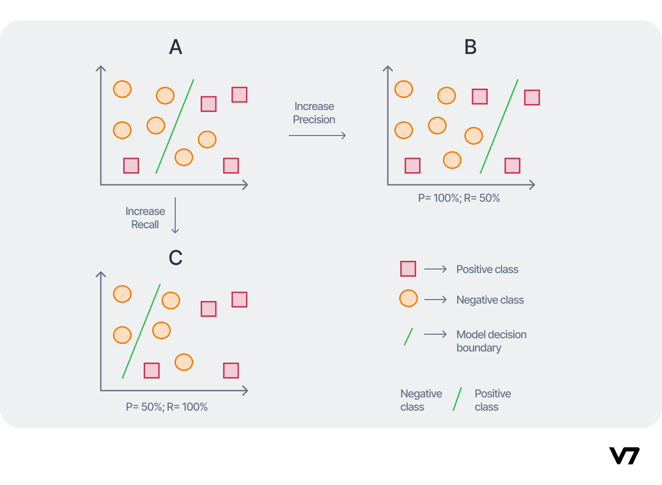
The Precision-Recall Trade-off
Improving precision often comes at the cost of recall, and vice-versa. A model can achieve 100% precision by being extremely conservative (e.g., only flagging an email as spam if it's 99.99% certain), but it will miss many borderline cases, lowering its recall. Conversely, a model can achieve 100% recall by being very aggressive (flagging anything that looks remotely like spam), but it will generate many false positives, lowering its precision.
F1-Score: The Harmonic Mean
The F1-score combines precision and recall into a single metric. It is the harmonic mean of the two.
The F1-score is useful when you want a balance between precision and recall, especially when you have an imbalanced dataset. It punishes extreme values more than a simple average. If either precision or recall is very low, the F1-score will also be low.
Test your understanding!
A model's confusion matrix yields the following: TP=80, FP=20, FN=40, TN=900.
- What is the precision?
- What is the recall?
- What is the F1-score?
Show answer
- Precision = TP / (TP + FP) = 80 / (80 + 20) = 80 / 100 = 0.8
- Recall = TP / (TP + FN) = 80 / (80 + 40) = 80 / 120 = 0.667
- F1-Score = 2 * (0.8 * 0.667) / (0.8 + 0.667) = 2 * 0.5336 / 1.467 = 0.727
Full Implementation from Scratch
Now, let's combine everything into a complete script. We will define functions for each metric and use them on the confusion matrix we created earlier.
import numpy as np

# --- Part 1: Our from-scratch functions ---

def create_confusion_matrix(y_true, y_pred):
    """Creates a confusion matrix. Assumes binary classification with labels 0 and 1."""
    # We'll stick to a 2x2 matrix for simplicity in this example
    cm = np.zeros((2, 2), dtype=int)
    for i in range(len(y_true)):
        cm[y_true[i], y_pred[i]] += 1
    return cm

def get_metrics_from_cm(cm):
    """Extracts TN, FP, FN, TP from a 2x2 confusion matrix."""
    tn, fp, fn, tp = cm[0, 0], cm[0, 1], cm[1, 0], cm[1, 1]
    return tn, fp, fn, tp

def precision(tp, fp):
    """Calculates precision."""
    # Add a small epsilon to avoid division by zero
    return tp / (tp + fp + 1e-8)

def recall(tp, fn):
    """Calculates recall."""
    return tp / (tp + fn + 1e-8)

def f1_score(prec, rec):
    """Calculates F1-score."""
    return 2 * (prec * rec) / (prec + rec + 1e-8)

# --- Part 2: Example Usage ---

# y_true: The ground truth labels
# y_pred: Predictions from a hypothetical model
y_true = np.array([1, 0, 1, 1, 0, 1, 0, 0, 1, 0, 1, 1, 0])
y_pred = np.array([1, 1, 1, 0, 0, 1, 0, 0, 1, 0, 0, 1, 1])

# 1. Create the confusion matrix
cm = create_confusion_matrix(y_true, y_pred)
print("From-scratch Confusion Matrix:")
print(cm)
print("-" * 30)

# 2. Extract TP, TN, FP, FN
# Assuming 1 is the positive class
tn, fp, fn, tp = get_metrics_from_cm(cm)
print(f"True Positives (TP): {tp}")
print(f"True Negatives (TN): {tn}")
print(f"False Positives (FP): {fp}")
print(f"False Negatives (FN): {fn}")
print("-" * 30)

# 3. Calculate metrics
prec = precision(tp, fp)
rec = recall(tp, fn)
f1 = f1_score(prec, rec)

print(f"Precision: {prec:.4f}")
print(f"Recall: {rec:.4f}")
print(f"F1-Score: {f1:.4f}")
print("-" * 30)

# --- Interpretation ---
print("Interpretation:")
print(f"Our model correctly identified {tp} out of the {tp+fn} actual positives (Recall = {rec:.2f}).")
print(f"When our model predicted an instance was positive, it was correct {prec:.2f} of the time (Precision = {prec:.2f}).")
From Learning to Practice: Using Scikit-Learn
While building these from scratch is excellent for understanding, in your projects, you'll use optimized, battle-tested library functions. scikit-learn provides a classification_report that gives you all these metrics instantly.
The following video shows how to use scikit-learn's tools to get these metrics and provides a great recap of the concepts.
All Binary Classification Metrics for ML - Implementing Precision, Recall, F1, & AUC in Python
To see how this is done in practice, watch this clip from Greg Hogg's tutorial. He implements these metrics and then shows the convenient classification_report.
Watch the following segments: 04:28 - 08:35: A clear walk-through of the confusion matrix and extracting TP, FP, FN, TN. 08:35 - 16:27: Implementation and explanation of Accuracy, Recall (True Positive Rate), Precision, and F1-score. 24:50 - 25:57: This final part shows how sklearn.metrics.classification_report provides a clean summary of all these metrics.
Using scikit-learn:
from sklearn.metrics import classification_report, confusion_matrix

# Use the same example data
y_true = np.array([1, 0, 1, 1, 0, 1, 0, 0, 1, 0, 1, 1, 0])
y_pred = np.array([1, 1, 1, 0, 0, 1, 0, 0, 1, 0, 0, 1, 1])

print("Scikit-learn Confusion Matrix:")
print(confusion_matrix(y_true, y_pred))
print("\nScikit-learn Classification Report:")
print(classification_report(y_true, y_pred, target_names=['Class 0 (Negative)', 'Class 1 (Positive)']))
Notice how the classification_report gives you precision, recall, and f1-score for each class, providing a comprehensive evaluation in one command.
Conclusion
You've now equipped yourself with the essential tools to properly evaluate any classification model. You not only understand the theory but have implemented the core metrics from scratch.
Key Takeaways:
- Accuracy is often a poor metric for classification, especially with imbalanced data.
- The confusion matrix is the starting point for a deeper analysis, breaking down predictions into True/False Positives/Negatives (TP, FP, FN, TN).
- Precision measures the quality of positive predictions (
TP / (TP + FP)). It's key when false positives are costly. - Recall measures the quantity of detected positives (
TP / (TP + FN)). It's key when false negatives are costly. - The F1-Score provides a single, balanced measure of a model's performance by taking the harmonic mean of precision and recall.
Preview of the Next Lesson:
We've thoroughly covered how to evaluate classification models. Now, we'll switch gears to the other major type of supervised learning: regression. In the next lesson, you will implement the calculation of regression metrics including Mean Squared Error (MSE) and R-squared, which are the standard metrics for evaluating how well a model predicts continuous values.