Stratified Sampling for Imbalanced Data Splitting

1. The Problem: Imbalance in Datasets

An imbalanced dataset is one where the classes are not represented equally. This is very common in real-world problems like:

• Fraud detection: The vast majority of transactions are legitimate, and only a tiny fraction are fraudulent.
• Medical diagnosis: Most patients tested may be healthy, with only a small number having the disease.
• Spam classification: Most emails might be non-spam ('ham'), with a smaller proportion being spam.

Here is a visual example of an imbalanced dataset for a binary classification task.

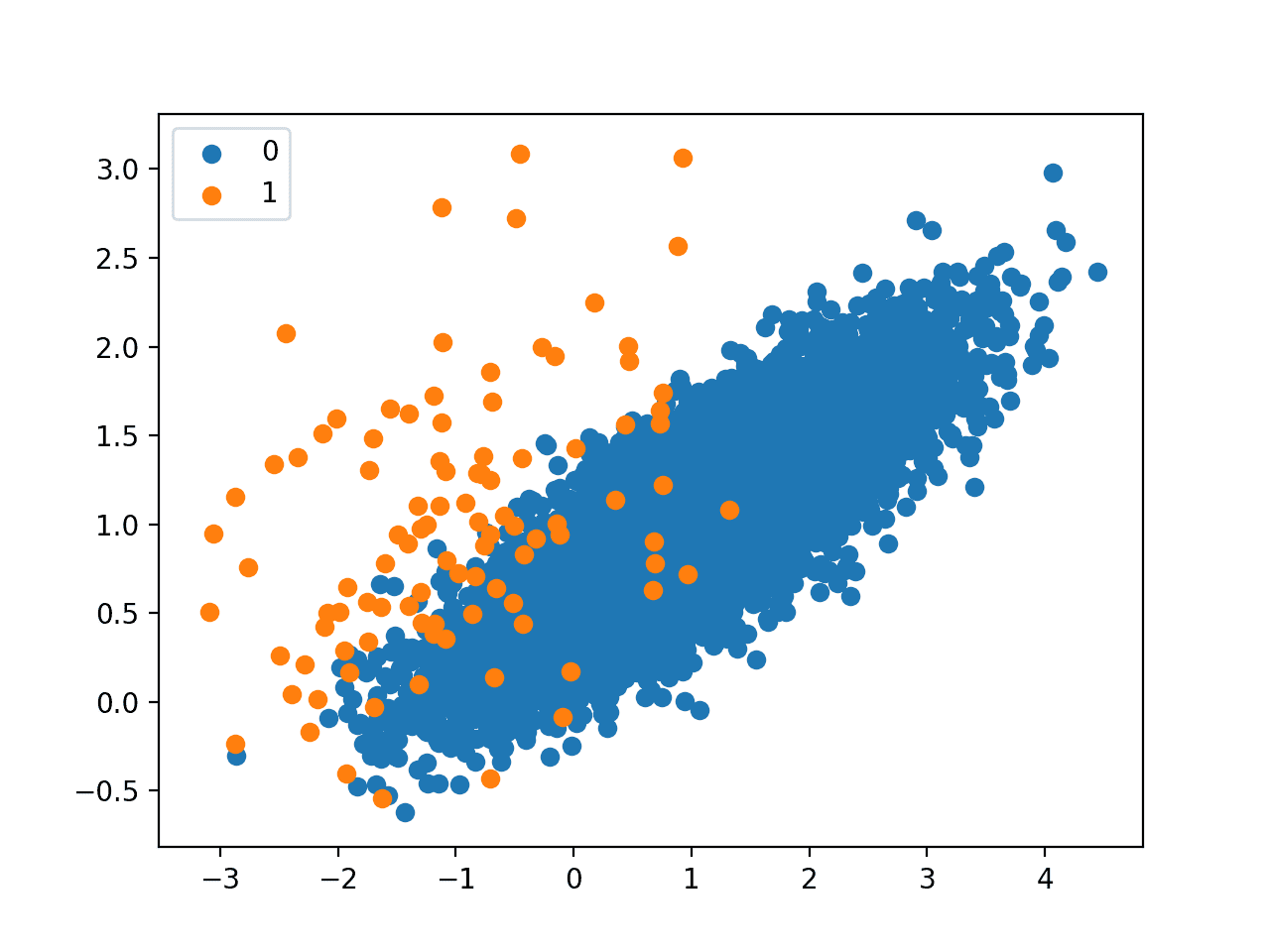
When we perform a simple random train-test split on such data, we might get an unrepresentative distribution. Imagine a dataset with 100 samples, where 90 belong to Class A and 10 to Class B. If we create a 20% test set, a random draw might accidentally place all 10 samples of Class B in the training set, leaving none for testing. The model would never be tested on its ability to predict Class B, leading to a misleading evaluation.

To understand this problem in a practical context, let's watch the first part of the following video, which demonstrates how a standard split can go wrong.

2. The Solution: Stratified Sampling

Stratified sampling solves this problem by enforcing a proportional split. The core idea is to divide the dataset into subgroups, or strata (in this case, by class label), and then draw samples from each subgroup to match the proportions of the original dataset.

This ensures that if Class B makes up 10% of the total dataset, it will also make up 10% of your training set and 10% of your test set.

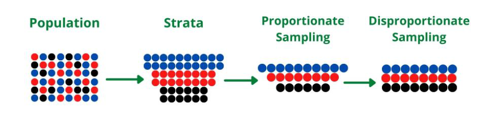
For a more detailed explanation of the concept, the following article provides an excellent breakdown of why simple random sampling can fail and how stratified sampling corrects for it.

3. Implementing Stratified Sampling from Scratch

In line with your preference for building from the ground up, we will now implement a stratified split function using Python and NumPy. Our function will take features X, labels y, and a test_size fraction, and return the four split datasets.

The logic of our implementation will be:

1. Identify the unique classes and find the indices corresponding to each class.
2. For each class, shuffle its indices and split them into training and testing portions based on the test_size.
3. Combine the indices from all classes to form the final training and testing index lists.
4. Shuffle the combined indices to ensure the data is not ordered by class.
5. Use these final index arrays to slice the original X and y data.

Here is the implementation:

import numpy as np
import pandas as pd # Used for easy verification

def stratified_train_test_split(X, y, test_size=0.2, random_state=None):
    """
    Performs a stratified train-test split on the given data.

    Args:
        X (np.ndarray): Feature data.
        y (np.ndarray): Target labels.
        test_size (float): The proportion of the dataset to include in the test split.
        random_state (int): Seed for the random number generator for reproducibility.

    Returns:
        A tuple containing (X_train, X_test, y_train, y_test).
    """
    if random_state is not None:
        np.random.seed(random_state)
        
    # 1. Get unique classes and their indices
    unique_classes, y_indices = np.unique(y, return_inverse=True)
    
    train_indices, test_indices = [], []
    
    # 2. Loop through each class
    for i in range(len(unique_classes)):
        # Find all indices belonging to the current class
        class_indices = np.where(y_indices == i)[0]
        
        # Shuffle the indices for this class
        np.random.shuffle(class_indices)
        
        # Calculate the number of test samples for this class
        n_test_samples = int(len(class_indices) * test_size)
        
        # Split the indices for this class
        class_test_indices = class_indices[:n_test_samples]
        class_train_indices = class_indices[n_test_samples:]
        
        # 3. Append to the main lists
        test_indices.extend(class_test_indices)
        train_indices.extend(class_train_indices)
        
    # 4. Shuffle the combined indices to mix classes
    np.random.shuffle(train_indices)
    np.random.shuffle(test_indices)
    
    # 5. Slice the original data
    X_train = X[train_indices]
    y_train = y[train_indices]
    X_test = X[test_indices]
    y_test = y[test_indices]
    
    return X_train, X_test, y_train, y_test

# --- Verification ---
# Create a highly imbalanced dataset
X_dummy = np.random.rand(1000, 2)
# 95% class 0, 5% class 1
y_dummy = np.array([0] * 950 + [1] * 50) 
np.random.shuffle(y_dummy) # Shuffle to make it realistic

# Apply our function
X_train, X_test, y_train, y_test = stratified_train_test_split(X_dummy, y_dummy, test_size=0.3, random_state=42)

# Check the results
print("Original dataset proportions:")
print(pd.Series(y_dummy).value_counts(normalize=True))
print("\nTraining set proportions:")
print(pd.Series(y_train).value_counts(normalize=True))
print("\nTest set proportions:")
print(pd.Series(y_test).value_counts(normalize=True))

When you run the code above, you'll see that the proportions of class 0 (95%) and class 1 (5%) are preserved almost perfectly across the original, training, and testing sets. This confirms our from-scratch implementation works as intended.

4. The Scikit-Learn Way

While implementing this from scratch provides deep insight, in practice you will often use scikit-learn's optimized functions. The train_test_split function you're familiar with has a stratify parameter that handles this automatically.

You just need to pass the target array y to this parameter, and scikit-learn takes care of the rest. The video from Stats Wire you watched earlier demonstrates this.

This is the standard, efficient way to perform a stratified split in most machine learning projects.

Conclusion

Congratulations on completing the first module! You have now built a comprehensive foundation for model evaluation and data preparation.

Key Takeaways from this Lesson:

• Imbalanced datasets are common and pose a risk of creating unrepresentative train/test splits.
• Stratified sampling is the solution, ensuring that class proportions are maintained across all data subsets.
• The from-scratch implementation involves splitting the data by class, sampling proportionally from each, and then recombining.
• In practice, sklearn.model_selection.train_test_split(..., stratify=y) is the go-to tool for this task.

Module 1 Wrap-Up:
You started this module by learning the fundamental distinctions in machine learning and have since built an impressive from-scratch toolkit. You can:

• Split data using train-test-validation and k-fold cross-validation.
• Handle imbalanced datasets with stratified sampling.
• Evaluate classification models with a confusion matrix, precision, recall, and F1-score.
• Assess regression models with MSE and R-squared.
• Visualize model trade-offs with ROC/AUC curves.
• Diagnose underfitting and overfitting with learning curves.

Preview of the Next Module:
With your evaluation toolkit complete, we can now shift our focus from assessing models to building them. The next module, "Optimization with Gradient Descent," will take you into the engine room of modern machine learning. In the first lesson, you will learn about the two core components that an optimizer needs to work: a loss function, which measures how wrong a model is, and the model's parameters, which are the knobs we can turn to make it better.