Visualizing Learning Curves for Model Diagnosis

1. Understanding Learning Curves

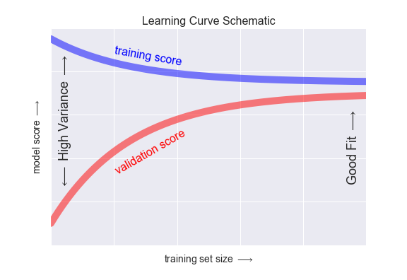
At its core, a learning curve is a plot that shows a model's performance as a function of the amount of training data. We typically plot two lines:

1. Training Score: The model's performance on the data it was trained on.
2. Validation Score: The model's performance on a separate, unseen set of data.

This allows us to see how well the model is learning (training score) and how well it's generalizing (validation score) as it gets more data.

To get a solid conceptual foundation, please watch the following video from a Cornell University course on Applied Machine Learning. It provides a clear and comprehensive explanation of learning curves.

Key Characteristics of Learning Curves

Based on the video, let's summarize the expected behavior:

• Training Error/Score:

  • When the training set is very small, the model can easily fit it perfectly, so the error is low (or score is high).
  • As the training set size increases, it becomes harder for the model to fit all the points perfectly, so the training error increases (or score decreases) and eventually plateaus.

• Validation Error/Score:

  • When the training set is very small, the model is poorly trained and can't generalize well, leading to high validation error (or a low score).
  • As the training set size increases, the model learns more robust patterns, so the validation error decreases (or score increases) and eventually plateaus.

2. Diagnosing Problems with Learning Curves

The real power of learning curves comes from interpreting the patterns they reveal about our model. The shapes of the curves and the gap between them are clear indicators of bias and variance.

The next segment of the same Cornell video explains exactly how to diagnose these issues.

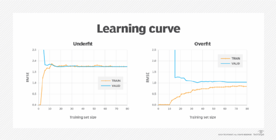
Here's a summary of the diagnostic patterns:

• High Bias (Underfitting):

  • Signature: Both the training and validation errors converge to a similarly high value.
  • Interpretation: The model is too simple to capture the underlying structure of the data. It performs poorly on both the training set and the validation set.
  • What to do: Adding more training data will not help. The curves have already plateaued. You need to use a more complex model (e.g., add polynomial features, use a more powerful algorithm) or add more informative features to the data.

• High Variance (Overfitting):

  • Signature: There is a large and persistent gap between the training and validation errors. The training error is low, while the validation error is much higher.
  • Interpretation: The model is too complex and is memorizing the training data, including its noise, instead of learning the general pattern. It fails to generalize to new data.
  • What to do: Adding more training data is likely to help. The validation curve is still decreasing, and more data will help the model learn a more generalizable pattern, shrinking the gap. Other solutions include reducing model complexity or applying regularization (which we'll cover later).

3. Implementing Learning Curves in Python

As you prefer, let's focus on the implementation. The general algorithm to generate learning curve data is:

1. Choose several different training set sizes.
2. For each size:
   a. Take a random subset of the training data of that size.
   b. Train your model on this subset.
   c. Evaluate the model on both the training subset and the full validation set.
   d. To make the results more robust, repeat this process several times (like in k-fold cross-validation) and average the scores.
3. Plot the averaged scores against the training set sizes.

Fortunately, scikit-learn has a built-in function, learning_curve, that handles this entire cross-validated procedure for us. It's an excellent tool that automates the logic we just described.

The following resource provides a great walkthrough of how to use this function and interpret its results, which we will use as a guide for our implementation.

Now, let's write a reusable Python function to generate and plot learning curves for any given model. We'll test it on synthetic data where we can control the complexity and clearly see the effects of underfitting and overfitting.

import numpy as np
import matplotlib.pyplot as plt
from sklearn.model_selection import learning_curve
from sklearn.linear_model import LinearRegression
from sklearn.preprocessing import PolynomialFeatures
from sklearn.pipeline import make_pipeline

def plot_learning_curve(estimator, title, X, y, ylim=None, cv=None, n_jobs=None, train_sizes=np.linspace(.1, 1.0, 5)):
    """
    Generate a simple plot of the test and training learning curve.
    """
    plt.figure(figsize=(10, 6))
    plt.title(title)
    if ylim is not None:
        plt.ylim(*ylim)
    plt.xlabel("Training examples")
    plt.ylabel("Score (R^2)")

    train_sizes, train_scores, test_scores = learning_curve(
        estimator, X, y, cv=cv, n_jobs=n_jobs, train_sizes=train_sizes, scoring='r2')
    
    train_scores_mean = np.mean(train_scores, axis=1)
    train_scores_std = np.std(train_scores, axis=1)
    test_scores_mean = np.mean(test_scores, axis=1)
    test_scores_std = np.std(test_scores, axis=1)

    plt.grid()

    plt.fill_between(train_sizes, train_scores_mean - train_scores_std,
                     train_scores_mean + train_scores_std, alpha=0.1, color="r")
    plt.fill_between(train_sizes, test_scores_mean - test_scores_std,
                     test_scores_mean + test_scores_std, alpha=0.1, color="g")
    
    plt.plot(train_sizes, train_scores_mean, 'o-', color="r", label="Training score")
    plt.plot(train_sizes, test_scores_mean, 'o-', color="g", label="Cross-validation score")

    plt.legend(loc="best")
    return plt

# --- Generate Synthetic Data ---
# A non-linear relationship that a simple linear model will fail to capture.
np.random.seed(0)
n_samples = 100
X = np.linspace(0, 10, n_samples).reshape(-1, 1)
y = np.sin(X).ravel() + np.random.randn(n_samples) * 0.5

# --- Case 1: Underfitting (High Bias) ---
# A simple linear model trying to fit a sine wave.
title = "Learning Curve (High Bias - Linear Regression)"
estimator_bias = LinearRegression()
plot_learning_curve(estimator_bias, title, X, y, ylim=(0.0, 1.01), cv=5)
plt.show()

# --- Case 2: Overfitting (High Variance) ---
# A very complex polynomial model (degree 15)
title = "Learning Curve (High Variance - Polynomial Degree 15)"
estimator_variance = make_pipeline(PolynomialFeatures(degree=15), LinearRegression())
plot_learning_curve(estimator_variance, title, X, y, ylim=(0.0, 1.01), cv=5)
plt.show()

# --- Case 3: Good Fit ---
# A polynomial model with a reasonable degree (4)
title = "Learning Curve (Good Fit - Polynomial Degree 4)"
estimator_good = make_pipeline(PolynomialFeatures(degree=4), LinearRegression())
plot_learning_curve(estimator_good, title, X, y, ylim=(0.0, 1.01), cv=5)
plt.show()

Interpreting the Plots:

• High Bias Plot: Notice how both the training and cross-validation scores converge to a low value. The model is too simple. Even with all the data, it can't achieve a good $R^2$ score. This is classic underfitting.
• High Variance Plot: Look at the huge gap between the red (training) and green (validation) curves. The training score is nearly perfect (1.0), but the validation score is much lower. The model has memorized the training data but fails to generalize. This is classic overfitting.
• Good Fit Plot: Here, both scores converge to a high value, and the gap between them is small. The training score is slightly higher, which is normal, but the model performs well on both seen and unseen data. This is what you aim for.

Conclusion

Congratulations on completing the first module! You've built a robust toolkit for model evaluation and diagnostics from scratch.

Key Takeaways from this Lesson:

• Learning curves plot model performance against training set size for both training and validation sets.
• They are a primary tool for diagnosing bias (underfitting) and variance (overfitting).
• High bias is identified when training and validation scores converge at a low level. The solution is to increase model complexity, not add more data.
• High variance is identified by a large gap between a high training score and a low validation score. The solution is often to add more data (if the curve hasn't plateaued), reduce model complexity, or use regularization.
• The sklearn.model_selection.learning_curve function is a practical and robust tool for generating this data using cross-validation.

Preview of the Next Module:
You now have a solid foundation for evaluating any supervised learning model you build. In the next module, we will shift gears from evaluation to construction. We'll start with the engine that drives most of machine learning: optimization. The next lesson will introduce the core concepts of optimization by explaining the role of a loss function and a model's parameters. This will set the stage for you to implement the famous gradient descent algorithm.