Benchmarking Your Algorithms

1. Architecting the "Algorithm Gauntlet"

Your existing pipeline with DataHandler, Model, and Trainer classes is the perfect foundation for this task. The goal now is to create a master script that orchestrates the entire evaluation process. This script will act as a "gauntlet," putting each of your algorithms through the same rigorous test on a given dataset.

The logical flow for your script will be:

1. Load Data: Choose one benchmark dataset (e.g., Breast Cancer) and load it.
2. Prepare Data: Use your DataHandler to perform the train-test split. You should also apply any necessary preprocessing, like feature scaling, which you implemented in Module 3.
3. Instantiate Models: Create a dictionary where keys are the model names (e.g., "Logistic Regression") and values are instances of your corresponding model classes, configured with sensible default hyperparameters.
4. Iterate, Train, Evaluate: Loop through your dictionary of models. In each iteration:
   • Instantiate your Trainer class with the current model and the data splits.
   • Run the training process.
   • Calculate the relevant performance metrics on the test set.
5. Collect Results: Store the metrics from each model in a structured way, such as a dictionary or a list of dictionaries, for later analysis.

Here is a Python code skeleton illustrating this structure. You will need to adapt it to the specific names of your classes and methods.

# --- 1. Imports ---
# Your model classes
from your_logistic_regression import LogisticRegression
from your_svm import SVM
from your_random_forest import RandomForest
from your_mlp import MLP
# ... import all other models you've built

# Your pipeline classes
from your_pipeline import DataHandler, Trainer

# Utility libraries
from sklearn.datasets import load_breast_cancer
import pandas as pd

# --- 2. Data Preparation ---
print("Loading and preparing the Breast Cancer dataset...")
X_raw, y_raw = load_breast_cancer(return_X_y=True)

# Use your DataHandler to split and scale the data
# Remember the importance of scaling for distance-based/gradient-based models!
data_handler = DataHandler(X_raw, y_raw)
X_train, y_train, X_test, y_test = data_handler.get_scaled_splits() # Assuming you have a method for this

# --- 3. Model Instantiation ---
# A dictionary to hold all your contenders
models_to_compare = {
    "Logistic Regression": LogisticRegression(learning_rate=0.01, n_iterations=1000),
    "Linear SVM": SVM(learning_rate=0.001, C=1.0, n_iters=1000), # Using C for soft margin
    "Random Forest": RandomForest(n_trees=20, max_depth=10, min_samples_split=2),
    "MLP": MLP(layer_dims=[X_train.shape[1], 20, 10, 1], learning_rate=0.01, num_iterations=500),
    # Add all your other models here:
    # "AdaBoost": AdaBoost(...),
    # "Gradient Boosting": GradientBoosting(...),
}

# --- 4. & 5. Training, Evaluation, and Collection ---
results = []
print("\nStarting the evaluation gauntlet...")
for name, model in models_to_compare.items():
    print(f"--- Training {name} ---")
    try:
        trainer = Trainer(model, X_train, y_train, X_test, y_test)
        trainer.train()
        metrics = trainer.evaluate() # Assuming this returns a dict like {'accuracy': 0.95, 'f1_score': 0.94}
        metrics['model'] = name
        results.append(metrics)
        print(f"✅ {name} evaluation complete.")
    except Exception as e:
        print(f"❌ Failed to train or evaluate {name}. Error: {e}")

# --- 6. Analysis (covered next) ---
results_df = pd.DataFrame(results)
print("\n--- Evaluation Complete ---")
print(results_df)

This script automates the core task of this lesson. Before running it, let's discuss how to present the results in a way that's easy to interpret.

2. Comparing and Visualizing Performance

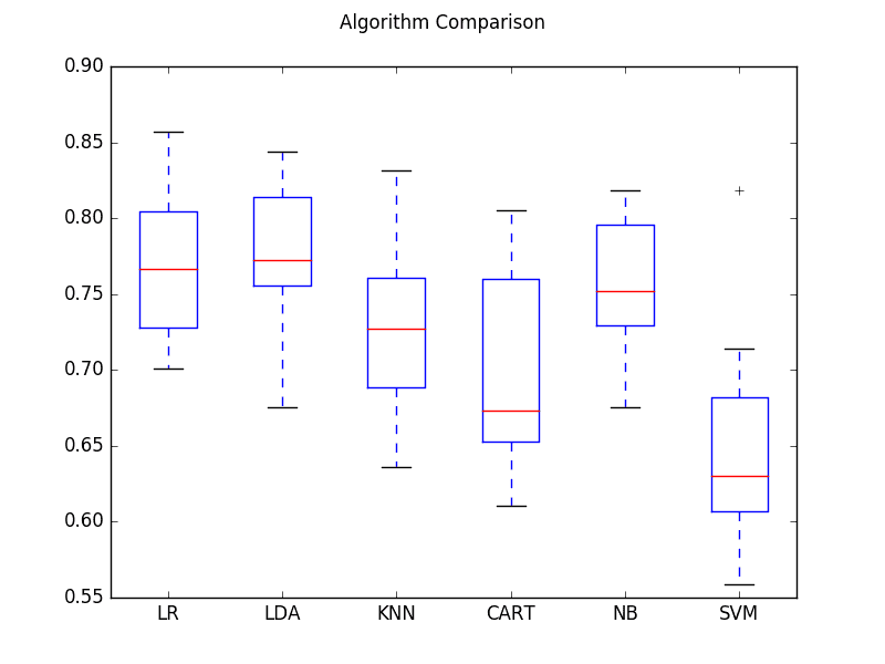
A table of numbers is a good start, but visualizations make the comparison immediate and intuitive. We want to quickly see which models are top performers and which are struggling.

The process of training a list of classifiers, gathering their scores, and plotting the results is a common task. The following video demonstrates this using Scikit-learn's built-in models, but the principle is identical to what you're doing with your from-scratch implementations.

As the video shows, a simple bar chart is highly effective for comparing a single key metric across all models. For your classification task on the Breast Cancer dataset, you could plot the F1-score. For your regression task on the California Housing data, you could plot the R-squared value or the inverse of MSE (since lower MSE is better).

3. Assembling the Final Report

Your final output for this task should be a report for each dataset (classification and regression) that includes:

1. A Performance Table: A pandas.DataFrame where rows represent your models and columns represent the key evaluation metrics you implemented in Module 1.
2. A Performance Chart: A bar chart comparing the primary metric (e.g., F1-score for classification, R-squared for regression) across all models.

Don't forget the metrics you've already implemented. For a quick refresher on them, you can consult this guide.

4. Advanced Comparison: Statistical Significance

For a true capstone-level analysis, simply observing that Model A has a higher score than Model B isn't enough. The difference might be due to random chance from the specific train-test split. A more rigorous approach involves statistical tests to determine if the performance difference is significant.

The Friedman Test followed by a post-hoc test (like the Nemenyi test) is a standard way to compare multiple algorithms across multiple datasets (or across multiple cross-validation folds on one dataset). The result is often visualized using a Critical Difference (CD) Diagram.

This is an advanced topic, but incorporating such a statistical test into your final report would demonstrate a deep understanding of rigorous model evaluation.

5. Professionalizing Your Workflow with sklearn.pipeline

Your current object-oriented pipeline is fantastic for understanding the mechanics of training. In many professional and production environments, this logic is encapsulated using Scikit-learn's Pipeline object. It chains together transformers (like your scaler) and an estimator (your model) into a single object.

This approach simplifies your training loop and reduces the risk of data leakage (e.g., fitting your scaler on the test set).

Considering your goal of working in SDE roles, mastering this pattern is extremely valuable. You could even consider refactoring your Trainer to work with sklearn.pipeline.Pipeline objects as an extension exercise.

Conclusion

This lesson has laid out the blueprint for the grand finale of your supervised learning course. You now have a clear plan to systematically run, evaluate, and compare every algorithm you have built. This process transforms your collection of individual models into a powerful comparative study.

Key Takeaways:

• A systematic evaluation can be automated with a script that iterates through models, trains them, and collects metrics.
• Your existing pipeline of DataHandler, Model, and Trainer classes is the perfect engine for this automation.
• Visualizations like bar charts are essential for quickly comparing model performance.
• A comprehensive analysis compares not just a single score, but also considers training time and model complexity.
• For advanced analysis, statistical tests like the Friedman test can determine if performance differences are significant.
• Scikit-learn's Pipeline object is the industry-standard tool for professionalizing this workflow.

Preview of the Next Lesson:
Your current evaluation uses default hyperparameters. But what if your SVM could perform better with a different C value, or your MLP with a different architecture? In the next lesson, you will tackle hyperparameter tuning, implementing logic to search for better model configurations using your validation set, further refining your model comparison.