Building Logistic Regression with Gradient Descent

1. Structuring the LogisticRegression Class

To build a reusable and organized model, we'll create a LogisticRegression class. This approach is standard practice and will make it easy to extend our model later (for example, when we add regularization). Our class will have a familiar structure:

• __init__(self, learning_rate, iterations): A constructor to set hyperparameters.
• fit(self, X, y): The training method that runs our gradient descent optimizer.
• predict(self, X): A method to make predictions on new, unseen data using the learned parameters.
• _sigmoid(self, z): A private helper method for the sigmoid calculation.

Let's start by defining the class structure. We'll initialize the weights and bias to None; they will be created and learned within the fit method.

import numpy as np

class LogisticRegression:
    def __init__(self, learning_rate=0.01, iterations=1000):
        self.lr = learning_rate
        self.iterations = iterations
        self.weights = None
        self.bias = 0

    def _sigmoid(self, z):
        return 1 / (1 + np.exp(-z))

    def fit(self, X, y):
        # We will implement this next
        pass

    def predict(self, X):
        # And we will implement this after fit
        pass

2. Implementing the Training Logic: The fit Method

The fit method is the heart of our model. It's where the learning happens. Inside this method, we will implement the vectorized gradient descent algorithm we derived in the previous lesson.

The following resource from GeeksForGeeks provides a very clean and direct implementation of a LogisticRegression class. We will use it as our guide.

Let's break down the implementation of the fit method from the article and connect it to our formulas.

1. Initialization: Before the loop, we get the number of samples (m) and features (n) from the input data X and initialize our weights vector to zeros.

   m, n = X.shape
   self.weights = np.zeros(n)
   self.bias = 0
   

2. The Gradient Descent Loop: We loop for the specified number of iterations. In each iteration, we perform one full step of gradient descent.

   for _ in range(self.iterations):
       # ... implementation inside the loop ...
   

3. Forward Pass: Inside the loop, we first calculate the model's predictions for all training examples at once.

   # Linear model: z = Xw + b
   z = np.dot(X, self.weights) + self.bias
   # Predicted probabilities: ŷ = σ(z)
   h = self._sigmoid(z) 
   

   Here, h corresponds to $\hat{Y}$, the vector of predicted probabilities.

4. Gradient Calculation: Next, we compute the gradients of the cost function with respect to the weights and bias using the vectorized formulas from our last lesson.

   • Formula for weights: $\frac{\partial J}{\partial w}=\frac{1}{m}{X}^T(\hat{Y}-Y)$

   • Code: dw = (1/m) * np.dot(X.T, (h - y))

   • Formula for bias: $\frac{\partial J}{\partial b}=\frac{1}{m}\sum ({\hat{y}}^{(i)}-y^{(i)})$

   • Code: db = (1/m) * np.sum(h - y)

   As you can see, the NumPy code is a direct and elegant translation of the mathematical formulas. This is the power of vectorization.

5. Parameter Update: Finally, we update the weights and bias by taking a step in the negative direction of the gradient.

   self.weights -= self.lr * dw
   self.bias -= self.lr * db
   

Putting it all together, our fit method looks like this:

def fit(self, X, y):
    m, n = X.shape
    self.weights = np.zeros(n)
    self.bias = 0

    # Gradient Descent
    for _ in range(self.iterations):
        # Forward pass
        z = np.dot(X, self.weights) + self.bias
        h = self._sigmoid(z)

        # Gradient calculation
        dw = (1/m) * np.dot(X.T, (h - y))
        db = (1/m) * np.sum(h - y)

        # Parameter update
        self.weights -= self.lr * dw
        self.bias -= self.lr * db

3. Implementing Predictions: The predict Method

Once the fit method has run, our model has learned the optimal weights and bias. Now, we can use them to make predictions on new data. The predict method will:

1. Calculate the predicted probabilities using the learned parameters.
2. Convert these probabilities into binary class labels (0 or 1) by applying a decision threshold of 0.5.

def predict(self, X):
    # Calculate probabilities
    z = np.dot(X, self.weights) + self.bias
    y_pred_proba = self._sigmoid(z)
    
    # Apply threshold to get class labels
    y_pred_class = (y_pred_proba >= 0.5).astype(int)
    return y_pred_class

The expression (y_pred_proba >= 0.5) returns a boolean array (True/False), which .astype(int) conveniently converts to 1s and 0s.

4. Training and Visualizing Your Model

Now for the exciting part: let's use our complete model. The following video provides a great walkthrough of the entire process, from loading data to training the model and, importantly, visualizing the result.

Let's try it ourselves. We will use the Breast Cancer dataset from scikit-learn, which you've seen in the resources.

First, let's gather our full class code in one place:

import numpy as np

class LogisticRegression:
    def __init__(self, learning_rate=0.01, iterations=1000):
        self.lr = learning_rate
        self.iterations = iterations
        self.weights = None
        self.bias = 0

    def _sigmoid(self, z):
        return 1 / (1 + np.exp(-z))

    def fit(self, X, y):
        m, n = X.shape
        self.weights = np.zeros(n)
        self.bias = 0

        for _ in range(self.iterations):
            z = np.dot(X, self.weights) + self.bias
            h = self._sigmoid(z)
            dw = (1/m) * np.dot(X.T, (h - y))
            db = (1/m) * np.sum(h - y)
            self.weights -= self.lr * dw
            self.bias -= self.lr * db

    def predict(self, X):
        z = np.dot(X, self.weights) + self.bias
        y_pred_proba = self._sigmoid(z)
        y_pred_class = (y_pred_proba >= 0.5).astype(int)
        return y_pred_class

Now, let's use it:

from sklearn.model_selection import train_test_split
from sklearn.datasets import load_breast_cancer
from sklearn.preprocessing import StandardScaler

# 1. Load and prepare data
data = load_breast_cancer()
X, y = data.data, data.target

# Split data
X_train, X_test, y_train, y_test = train_test_split(X, y, test_size=0.2, random_state=42)

# Scale features - very important for gradient descent!
scaler = StandardScaler()
X_train = scaler.fit_transform(X_train)
X_test = scaler.transform(X_test)

# 2. Train our model
model = LogisticRegression(learning_rate=0.1, iterations=1000)
model.fit(X_train, y_train)

# 3. Evaluate the model
predictions = model.predict(X_test)
accuracy = np.mean(predictions == y_test)
print(f"Model Accuracy: {accuracy * 100:.2f}%")

# Expected Output (may vary slightly):
# Model Accuracy: 98.25%

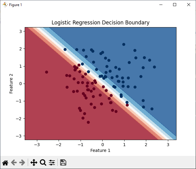
The result of your trained model is a decision boundary, a line or surface that separates the different classes. For a 2D dataset, it looks like this:

Conclusion

Congratulations! You have successfully built and trained a complete logistic regression classifier from scratch. You translated the mathematical formulas for gradient descent into a working, vectorized Python implementation.

Key Takeaways:

• Structuring your model in a class (__init__, fit, predict) makes your code organized, reusable, and similar to industry-standard libraries.
• The fit method is a direct implementation of the gradient descent loop, iteratively updating model weights and bias based on the calculated gradients.
• Vectorization with NumPy is crucial for an efficient implementation, allowing you to process the entire dataset without explicit for loops.
• The predict method uses the final learned parameters to estimate probabilities and classify new data points based on a decision threshold.

Preview of the Next Lesson:
Seeing is believing. While you've printed the accuracy, visualizing the decision boundary provides deeper insight into how your model is separating the data. In the next lesson, we will focus specifically on visualizing the decision boundary of your trained logistic regression model on a 2D dataset to better understand its behavior.