Gradient of Binary Cross-Entropy Loss

Hello! Welcome to the next lesson in our journey through supervised learning.

In the last lesson, you successfully implemented the sigmoid function, our tool for converting a linear model's output into a probability between 0 and 1. We now have a way to make a prediction: given an input $x$ , we can compute a linear score $z = θ^{T} x + b$ and then find the predicted probability $y^= σ (z)$ .

But how do we know if our prediction $y^$ is any good? And more importantly, how can we systematically improve our model's parameters, $θ$ and $b$ , to make better predictions? To answer these questions, we need a loss function that quantifies the error between our prediction $y^$ and the true label $y$ .

Today, we will dive into the binary cross-entropy loss function, the standard for binary classification tasks. Our main goal is to derive and calculate its gradient. This gradient is the crucial signal that will tell our gradient descent optimizer how to adjust the model's parameters to minimize the error.

1. Quantifying Error with Binary Cross-Entropy

For linear regression, we used Mean Squared Error (MSE), which measures the average squared distance between predicted and true values. For classification, the problem is different. We are predicting probabilities, not continuous values.

The loss function for logistic regression is called Binary Cross-Entropy (BCE), or log loss. For a single training example, it's defined as:

L (y^, y) = - [y lo g (y^) + (1 - y) lo g (1 - y^)]

Let's break down why this works:

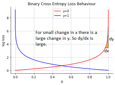
Case 1: True label $y = 1$
The formula simplifies to $L = - lo g (y^)$ . If our prediction $y^$ is close to 1 (e.g., 0.99), $lo g (y^)$ is close to 0, so the loss is very small. If $y^$ is close to 0 (e.g., 0.01), $lo g (y^)$ is a large negative number, so the loss becomes very large. The model is heavily penalized for being confidently wrong.
Case 2: True label $y = 0$
The formula simplifies to $L = - lo g (1 - y^)$ . If our prediction $y^$ is close to 0, then $1 - y^$ is close to 1, and the loss is small. If $y^$ is close to 1, then $1 - y^$ is close to 0, and the loss becomes very large. Again, the model is penalized for being wrong.

This plot visualizes the behavior perfectly.

Binary Cross-Entropy Loss Behavior and Gradient — This plot shows the binary cross-entropy loss for a true label of y=1 (blue curve) and y=0 (red curve). For y=1, the loss skyrockets as the predicted probability approaches 0. For y=0, the loss skyrockets as the prediction approaches 1. The steepness of the curve is the gradient, which our optimizer will use.

The total cost over the entire training set of $m$ examples is simply the average of the individual losses:

J (θ, b) = \frac{1}{m} i = 1 \sum m L (y^^{(i)}, y^{(i)}) = - \frac{1}{m} i = 1 \sum m [y^{(i)} lo g (y^^{(i)}) + (1 - y^{(i)}) lo g (1 - y^^{(i)})]

Our goal is to find the parameters $θ$ (or weights $w$ ) and $b$ that minimize this cost function $J$ .

2. Deriving the Gradient of the Loss Function

To use gradient descent, we need to compute the partial derivatives of the cost function $J$ with respect to each parameter. Let's focus on a single parameter $w_{j}$ (a single weight in our weight vector) and the bias $b$ . For simplicity, let's consider the loss for a single training example, $L$ .

We'll use the chain rule, which is fundamental to how neural networks are trained. You'll see it again when we cover backpropagation. Our variables are linked like this:

A linear combination: $z = w^{T} x + b$
The sigmoid activation: $y^= σ (z)$
The loss: $L = - [y lo g (y^) + (1 - y) lo g (1 - y^)]$

To find $\frac{\partial L}{\partial w _{j}}$ , we can chain the derivatives together:

\frac{\partial L}{\partial w _{j}} = \frac{\partial L}{\partial y ^} \cdot \frac{\partial y ^}{\partial z} \cdot \frac{\partial z}{\partial w _{j}}

Let's derive each piece. The following reading provides an excellent, step-by-step derivation.

Logistic Regression Model from Scratch

This article, 'Logistic Regression Model from Scratch', contains a clear derivation of the gradient using the chain rule. We'll follow its logic closely.

Read the section titled 'Gradient Descent' up to equation (13). Focus on how the author breaks down the problem using the chain rule into three smaller derivatives and then combines them at the end. Don't worry about the vector notation (∇) for now; we'll focus on the single-variable derivatives first.

Let's re-create that derivation here to solidify our understanding.

Step 1: Derivative of Loss w.r.t. Prediction ( $\frac{\partial L}{\partial y ^}$ )

\frac{\partial L}{\partial y ^} = \frac{\partial}{\partial y ^} (- [y lo g (y^) + (1 - y) lo g (1 - y^)]) = - (\frac{y}{y ^} - \frac{1 - y}{1 - y ^}) = \frac{y ^ - y}{y ^ ( 1 - y ^ )}

Step 2: Derivative of Sigmoid w.r.t. its Input ( $\frac{\partial y ^}{\partial z}$ )

This is a classic derivative. The derivative of $σ (z)$ has a neat form:

\frac{\partial y ^}{\partial z} = \frac{\partial}{\partial z} σ (z) = σ (z) (1 - σ (z)) = y^(1 - y^)

Step 3: Derivative of Linear Combination w.r.t. a Weight ( $\frac{\partial z}{\partial w _{j}}$ )

Given $z = w_{1} x_{1} + w_{2} x_{2} + ... + w_{j} x_{j} + ... + w_{n} x_{n} + b$ , the partial derivative with respect to $w_{j}$ is simply its corresponding feature value, $x_{j}$ .

\frac{\partial z}{\partial w _{j}} = x_{j}

Putting It All Together

Now, we multiply the three parts:

\frac{\partial L}{\partial w _{j}} = (\frac{y ^ - y}{y ^ ( 1 - y ^ )}) \cdot (y^(1 - y^)) \cdot (x_{j})

The $y^(1 - y^)$ terms cancel out, leaving us with a wonderfully simple result:

\frac{\partial L}{\partial w _{j}} = (y^- y) x_{j}

This result is elegant and intuitive. The gradient for a weight $w_{j}$ is the prediction error $(y^- y)$ multiplied by the corresponding input feature $x_{j}$ . If the error is large, the gradient is large, leading to a bigger update.

For the bias term, $b$ , the derivation is similar, but since $\frac{\partial z}{\partial b} = 1$ , the final gradient is just the error term:

\frac{\partial L}{\partial b} = y^- y

Test your understanding!

Looking at the final gradient formula $\frac{\partial L}{\partial w _{j}} = (y^- y) x_{j}$ , what happens to the gradient if the model's prediction $y^$ is perfect (i.e., $y^= y$ )? What does this imply for the gradient descent update step?

Show answer

If the prediction is perfect, the error term $(y^- y)$ becomes zero. This makes the entire gradient $\frac{\partial L}{\partial w _{j}}$ equal to zero. In the gradient descent update step ( $w_{j} := w_{j} - α \frac{\partial L}{\partial w _{j}}$ ), this means the weight $w_{j}$ will not be updated at all, because we are already at a point of minimum loss for that specific training example.

3. Vectorizing the Gradient Calculation

Performing these calculations one example and one feature at a time is inefficient. Given your experience with NumPy, you know that vectorization is the key to performance. Let's see how to compute the gradients for all parameters across all $m$ training examples in one go.

The cost function gradient, averaged over all $m$ examples, can be written in matrix form.

Let $X$ be the design matrix of shape ( $m, n$ ), where $m$ is the number of examples and $n$ is the number of features.
Let $Y$ be the vector of true labels of shape ( $m, 1$ ).
Let $Y^$ be the vector of predicted probabilities of shape ( $m, 1$ ).
Let $w$ be the weight vector of shape ( $n, 1$ ).

The vectorized gradients are:

$\frac{\partial J}{\partial w} = \frac{1}{m} X^{T} (Y^- Y)$
$\frac{\partial J}{\partial b} = \frac{1}{m} \sum_{i = 1}^{m} (y^^{(i)} - y^{(i)})$

This matrix multiplication $X^{T} (Y^- Y)$ might seem abstract, but it's just a compact way of computing $(y^^{(i)} - y^{(i)}) x_{j}^{(i)}$ for all $i$ and $j$ and summing them up correctly.

The following video from the DeepLearningAI course by Andrew Ng provides an excellent explanation of how this vectorization works in practice.

Vectorizing Logistic Regression's Gradient Computation (C1W2L14)

This video breaks down how to transition from a for loop over training examples to a fully vectorized implementation for computing the gradients.

Watch the entire video (from 00:35 to 08:22). Pay close attention to how the individual dz terms are stacked into a vector DZ, and how matrix multiplication (X * DZ.T) is used to compute the final dw gradient vector without any explicit loops. This is a core concept you will use when implementing logistic regression.

To summarize the key idea from the video, the steps for one iteration of gradient descent are:

Forward Pass (Vectorized):
- Z = np.dot(X, w) + b (or w.T @ X if w is a row vector)
- A = sigmoid(Z) (Here A is $Y^$ )
Backward Pass / Gradient Calculation (Vectorized):
- dZ = A - Y
- dw = (1/m) * np.dot(X.T, dZ)
- db = (1/m) * np.sum(dZ)
Parameter Update:
- w = w - learning_rate * dw
- b = b - learning_rate * db

This sequence of operations is exactly what you will implement in the next lesson to build your logistic regression classifier.

Conclusion

In this lesson, we bridged the gap between making a prediction and learning from our errors. You now understand the "engine" of logistic regression.

Key Takeaways:

Binary Cross-Entropy is the loss function used to measure the error in binary classification models. It heavily penalizes confident but incorrect predictions.
Using the chain rule, we derived the gradient of the loss function with respect to the model's parameters.
The gradient for a single weight $w_{j}$ has the simple and intuitive form: (prediction_error) × (input_feature), or $(y^- y) x_{j}$ .
Vectorization allows us to compute these gradients efficiently across the entire dataset with a few lines of NumPy code, avoiding slow Python loops. The key formulas are $\frac{\partial J}{\partial w} = \frac{1}{m} X^{T} (Y^- Y)$ and $\frac{\partial J}{\partial b} = \frac{1}{m} \sum (Y^- Y)$ .

Preview of the Next Lesson:
You are now fully equipped! You have the sigmoid function to make predictions and the vectorized gradient of the loss function to guide the learning process. In the next lesson, you will put all the pieces together and implement a complete binary logistic regression model from scratch using your gradient descent optimizer.

Recommended resources

1. Quantifying Error with Binary Cross-Entropy

2. Deriving the Gradient of the Loss Function

3. Vectorizing the Gradient Calculation

Conclusion