Building a Gradient Boosting Regressor

The Gradient Boosting Algorithm: A Step-by-Step Guide

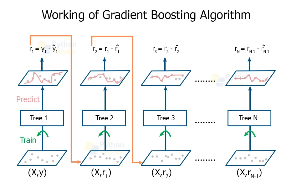
At its heart, Gradient Boosting for regression is an iterative process. You start with a very basic guess and then sequentially add "corrections" to it. Each correction is a small decision tree trained to fix the errors that remain.

This entire process can be broken down into a clear algorithm:

1. Initialize the model's prediction, $F_0(x)$. For regression with MSE loss, the best starting point is a constant value that minimizes the initial error. This value is simply the mean of all the target values, y. So, for every sample, our first prediction is $\bar{y}$.

2. Iterate from m = 1 to M (where M is the total number of trees):
   a. Calculate pseudo-residuals. For each sample, compute the error of the current ensemble:
   $r_{im}=y_i-F_{m-1}(x_i)$
   Here, $F_{m-1}(x_i)$ is the prediction for sample $i$ from the ensemble of all previous trees.

   b. Fit a weak learner. Train a new regression decision tree, $h_m(x)$, using the original features $X$ as input and the pseudo-residuals $\{r_{i1},...,r_{iN}\}$ as the target variable. This tree learns to predict the errors of the current model.

   c. Update the ensemble prediction. Add the new tree's contribution to the overall model, scaled by a learning rate, $\eta$:
   $F_m(x)=F_{m-1}(x)+\eta \cdot h_m(x)$
   The learning rate shrinks the contribution of each tree, which has been shown to improve the model's generalization.

3. Output the final model, $F_M(x)$. The final prediction is the sum of the initial prediction and the contributions of all M trees.

The following diagram provides a great visual summary of this sequential error-correcting process.

The following video provides a detailed, step-by-step walkthrough of this exact algorithm with concrete numbers. It's an excellent resource for solidifying your understanding before we jump into the code.

Implementing the Gradient Boosting Regressor

Now, let's translate this algorithm into a Python class. Since you've already implemented a decision tree, we can use sklearn.tree.DecisionTreeRegressor as our weak learner. This allows us to focus purely on the boosting logic that orchestrates the ensemble.

The article "Lesson 5 - Gradient boosting deep dive" provides a clear and concise implementation that we will follow. It builds a class named LSBoost (for Least-Squares Boost), which is exactly what we're aiming for.

Let's build our GradientBoostingRegressor class step-by-step.

1. The Class Structure

We'll start with an __init__ method to store hyperparameters and a list for our weak learners (the trees).

import numpy as np
from sklearn.tree import DecisionTreeRegressor

class GradientBoostingRegressor:
    """
    A Gradient Boosting Regressor implemented from scratch.
    
    Uses DecisionTreeRegressor as the weak learner.
    """
    def __init__(self, n_estimators=100, learning_rate=0.1, max_depth=3):
        self.n_estimators = n_estimators
        self.learning_rate = learning_rate
        self.max_depth = max_depth
        self.trees = []
        self.initial_prediction_ = None # To store the F_0 prediction

2. The fit Method

This is the core of the algorithm. It will initialize the prediction and then loop through n_estimators, creating and fitting a new tree in each iteration.

# We'll add this method to our GradientBoostingRegressor class.

def fit(self, X, y):
    """
    Fits the gradient boosting model.
    
    Args:
        X (np.array): Training data of shape (n_samples, n_features).
        y (np.array): Target values of shape (n_samples,).
    """
    # 1. Initialize the model's prediction
    self.initial_prediction_ = np.mean(y)
    current_predictions = np.full(shape=y.shape, fill_value=self.initial_prediction_)

    # 2. Iterate M times
    for _ in range(self.n_estimators):
        # 2a. Calculate pseudo-residuals
        residuals = y - current_predictions
        
        # 2b. Fit a weak learner (decision tree)
        tree = DecisionTreeRegressor(max_depth=self.max_depth)
        tree.fit(X, residuals)
        
        # 2c. Update the ensemble prediction
        # Get predictions from the newly trained tree
        update = tree.predict(X)
        # Add the update to our current predictions, scaled by the learning rate
        current_predictions += self.learning_rate * update
        
        # Store the trained tree
        self.trees.append(tree)

# Let's attach the fit method to our class
GradientBoostingRegressor.fit = fit

3. The predict Method

Once the model is fitted, making predictions on new data is straightforward. We start with the same initial prediction and then add the scaled contributions from all the trees we've stored.

# We'll also add this method to our class.

def predict(self, X):
    """
    Makes predictions on new data.
    
    Args:
        X (np.array): Data to predict on of shape (n_samples, n_features).
        
    Returns:
        np.array: The predicted values.
    """
    # Start with the initial constant prediction
    # We need to create an array of the correct shape
    y_pred = np.full(shape=X.shape[0], fill_value=self.initial_prediction_)
    
    # Add the contribution of each tree in the ensemble
    for tree in self.trees:
        y_pred += self.learning_rate * tree.predict(X)
        
    return y_pred

# Attach the predict method
GradientBoostingRegressor.predict = predict

Putting It All Together

Now you have a complete implementation. Let's see it in action on a simple dataset.

# --- Example Usage ---

# Generate a noisy quadratic dataset
np.random.seed(42)
X = np.random.rand(100, 1) - 0.5
y = 3 * X[:, 0]**2 + 0.05 * np.random.randn(100)

# Instantiate and train our model
gbr = GradientBoostingRegressor(n_estimators=100, learning_rate=0.1, max_depth=2)
gbr.fit(X, y)

# Make predictions
y_pred = gbr.predict(X)

# You can now plot y_pred against X to see how well it learned the curve!
import matplotlib.pyplot as plt

plt.figure(figsize=(10, 6))
plt.scatter(X, y, label='Original Data')
# Sort values for plotting the line correctly
sorted_zip = sorted(zip(X.flatten(), y_pred))
X_sorted, y_pred_sorted = zip(*sorted_zip)
plt.plot(X_sorted, y_pred_sorted, color='r', label='GBR Prediction')
plt.title('Gradient Boosting Regressor from Scratch')
plt.xlabel('X')
plt.ylabel('y')
plt.legend()
plt.show()

This implementation brings together everything we've discussed. It starts with a simple model and iteratively refines it by fitting trees to the remaining errors, just as you saw in the StatQuest video and the hepml article.

Conclusion

Congratulations! You have successfully implemented a complete Gradient Boosting Regressor from scratch. This is a significant achievement that builds upon several concepts from our course.

Key Takeaways:

• The Gradient Boosting algorithm for regression initializes with a mean prediction and then sequentially fits decision trees to the pseudo-residuals of the current ensemble.
• The fit method implements the core training loop: calculate residuals, fit a tree, and update the aggregate prediction.
• The predict method generates predictions by summing the initial prediction and the scaled outputs of all trained trees.
• By using a pre-existing DecisionTreeRegressor as a weak learner, we can focus on the boosting logic, which is the key to the algorithm's power.

Preview of the Next Module:
We have now concluded our deep dive into tree-based ensemble methods. In the next module, "Neural Network Foundations," we will shift gears dramatically. You will begin your journey into deep learning by implementing the fundamental building blocks of neural networks from scratch. Our first lesson will focus on implementing and visualizing common activation functions like Sigmoid, Tanh, and ReLU.