Calculating Pseudo-Residuals for Regression Loss Functions

From Simple Errors to Pseudo-Residuals

Let's start with a simple regression problem. The most intuitive way to measure error is to calculate the residual: the difference between the actual value and the predicted value.

Residual = Actual Value - Predicted Value

The core idea of Gradient Boosting for regression is to build a sequence of models, where each new model is trained to predict the residuals of the previous one.

The following video provides a great high-level overview of this process. It shows how we start with a simple initial prediction and then iteratively build trees to correct the remaining errors (residuals).

This iterative process can be visualized as a pipeline where each new model works to shrink the errors left by the previous ones.

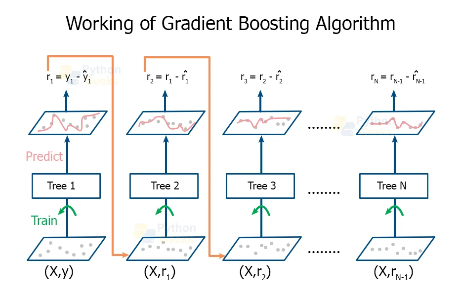
As you saw in the video, the term pseudo-residual was used. Why not just "residual"? Because this process is part of a more general framework that connects directly to gradient descent.

The "Gradient" in Gradient Boosting

The name "Gradient Boosting" isn't a coincidence. The algorithm is a form of gradient descent, but with a twist. In standard gradient descent, we update a model's parameters by moving them in the direction of the negative gradient of the loss function.

In Gradient Boosting, we are performing a similar optimization, but instead of updating parameters, we are adding a whole new function (a weak learner) to our ensemble. The goal of this new function is to move our overall prediction in the direction of the negative gradient of the loss function.

The "error" that we fit each new tree to is precisely this negative gradient of the loss function with respect to the previous prediction. This is the formal definition of a pseudo-residual.

Let's see this in action for the Mean Squared Error (MSE) loss function, which is commonly scaled by 1/2 for mathematical convenience.
The loss for a single data point is:

where $y$ is the true value and $\hat{y}$ is the current prediction.

The pseudo-residual is the negative gradient of this loss with respect to the prediction $\hat{y}$:

Let's calculate that gradient using the chain rule:

So, the pseudo-residual is:

For MSE, the pseudo-residual is exactly the same as the ordinary residual!

This is a crucial insight. The intuitive idea of fitting to residuals is mathematically grounded in the principle of gradient descent in function space. The following video explains this connection very clearly.

Implementing the Calculation

Now let's translate this into code. Your goal for this lesson is to be able to calculate these pseudo-residuals. Given an array of true values y and an array of the model's current predictions y_pred, calculating the pseudo-residuals for MSE is straightforward.

The article "Gradient boosting deep dive" provides a clean implementation of a LeastSquares loss class that includes a gradient method. Note that their gradient method returns -(y - y_pred). The pseudo-residual is the negative of this gradient.

Let's write a simple Python function to do this.

import numpy as np

def calculate_mse_pseudo_residuals(y_true, y_pred):
    """
    Calculates the pseudo-residuals for the Mean Squared Error loss function.

    Args:
        y_true (np.array): The true target values.
        y_pred (np.array): The current predictions of the model.

    Returns:
        np.array: The pseudo-residuals.
    """
    # For MSE, the pseudo-residual is simply the residual.
    return y_true - y_pred

# --- Example ---
# True values
y = np.array([150, 165, 180, 172])

# Initial prediction (e.g., the mean of y)
initial_prediction = np.mean(y)
y_pred_0 = np.full(shape=y.shape, fill_value=initial_prediction)

print(f"True values: {y}")
print(f"Initial predictions: {y_pred_0}")

# Calculate the first set of pseudo-residuals
residuals_0 = calculate_mse_pseudo_residuals(y, y_pred_0)
print(f"Pseudo-residuals for the first tree: {residuals_0}")

# In the next lesson, we would train a decision tree on these residuals.
# Let's assume that tree predicts the following values for our residuals:
tree_1_preds = np.array([-15, -2, 12, 5])

# We update our predictions
learning_rate = 0.1
y_pred_1 = y_pred_0 + learning_rate * tree_1_preds
print(f"\nUpdated predictions: {y_pred_1}")

# Now we calculate the *new* pseudo-residuals for the next tree to fit
residuals_1 = calculate_mse_pseudo_residuals(y, y_pred_1)
print(f"Pseudo-residuals for the second tree: {residuals_1}")

This image shows this exact calculation happening inside a fit method.

Beyond MSE: The Power of Generality

So, why bother with the term "pseudo-residual" if it's just the residual for MSE? Because for other loss functions, the negative gradient is not the simple residual. The ability to swap out the loss function is what makes Gradient Boosting so versatile.

For example, if we use the Absolute Error loss function, $L=|y-\hat{y}|$:

• The gradient $\frac{\partial L}{\partial \hat{y}}$ is $\text{sign}(\hat{y}-y)$, which is -1 if $\hat{y}<y$ and +1 if $\hat{y}>y$.
• The pseudo-residual (the negative gradient) is $\text{sign}(y-\hat{y})$.

This is no longer the simple residual, but our algorithm doesn't care. It will happily fit a tree to these new values of +1 and -1. This is the power of the framework. You can explore the pseudo-residuals for different loss functions in the "Pseudo-residuals again" section of the Statlect article.

Conclusion

In this lesson, you've grasped a fundamental concept that underpins one of the most powerful machine learning algorithms.

Key Takeaways:

• Gradient Boosting is an ensemble method that sequentially fits new models to correct the "errors" of the previous ones.
• These "errors" are formally called pseudo-residuals.
• A pseudo-residual is defined as the negative gradient of the loss function with respect to the model's current prediction.
• For the common case of Mean Squared Error (MSE) in regression, the pseudo-residual simplifies to the ordinary residual: actual value - predicted value.
• This framework allows any differentiable loss function to be used, making Gradient Boosting a highly flexible and powerful technique.

Preview of the Next Lesson:
You now know how to calculate the target that each new tree in our ensemble should predict. In the next lesson, "Implement a Gradient Boosting Regressor by iteratively fitting decision trees to pseudo-residuals," we will put this knowledge into action. You'll build the full training loop from scratch, combining your DecisionTree implementation with the pseudo-residual calculation to create a complete Gradient Boosting model.