Decision Stumps as Weak Learners

From Strong Learners to Weak Learners

In the last module, we built deep decision trees. A single, unconstrained decision tree is considered a strong learner because it can be made arbitrarily complex to fit the training data very closely (often leading to overfitting). Random Forests combine many of these strong learners in a way that reduces variance.

Boosting takes the opposite approach. It starts with weak learners: models that are only slightly better than random guessing. A weak learner has high bias but low variance. The core idea of boosting is that by combining many weak learners in a clever, sequential way, we can produce a single, highly accurate strong learner.

The most common and intuitive weak learner is the decision stump.

What is a Decision Stump?

A decision stump is a decision tree with a maximum depth of one. It consists of a single root node that splits the data directly into two leaf nodes. It makes its decision based on a single feature and a single threshold value.

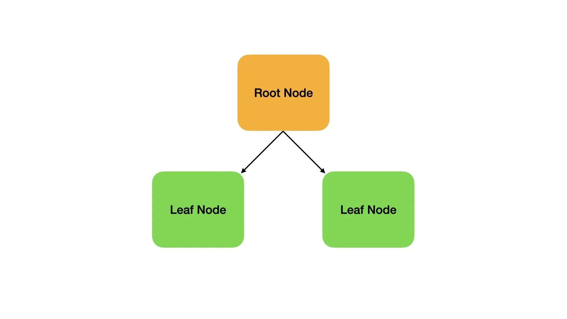
Given your experience building a recursive DecisionTree class, you can think of a decision stump as simply setting max_depth=1 in your previous implementation. However, for boosting algorithms, it's often more efficient and conceptually clearer to create a dedicated, lightweight DecisionStump class. This also allows us to introduce concepts like "polarity," which will be useful later.

To understand the concept of a weak learner and a decision stump in the context of boosting, let's turn to a short video and an article.

Implementing a Decision Stump Class

Let's build our DecisionStump class from scratch. It needs to store three key pieces of information that define the split:

1. feature_idx: The index of the feature to split on.
2. threshold: The value of the feature to use for the split.
3. polarity: Determines the classification of samples on either side of the threshold. For example, a polarity of 1 might mean "samples < threshold are class -1," while a polarity of -1 would flip this to "samples > threshold are class -1." This gives the stump flexibility to handle different feature distributions.

We'll also need a predict method that applies this rule to new data. For consistency with boosting algorithms like AdaBoost, we'll assume our class labels are +1 and -1.

Here is the full implementation.

import numpy as np

class DecisionStump:
    """
    A Decision Stump is a decision tree with a depth of one.
    It splits the data based on a single feature and a single threshold.
    """
    def __init__(self):
        # Polarity indicates whether samples < threshold are classified as -1 or +1
        self.polarity = 1
        # The index of the feature used for the split
        self.feature_idx = None
        # The threshold value for the feature
        self.threshold = None
        # The weight of this stump in the final ensemble (used in AdaBoost)
        self.alpha = None

    def predict(self, X):
        """
        Predicts the class labels for a given set of samples.
        """
        n_samples = X.shape[0]
        # Select the column for the chosen feature
        X_column = X[:, self.feature_idx]

        # Start by predicting +1 for all samples
        predictions = np.ones(n_samples)

        # Apply the stump rule based on polarity
        if self.polarity == 1:
            # If feature value is less than threshold, predict -1
            predictions[X_column < self.threshold] = -1
        else:
            # If feature value is greater than threshold, predict -1
            predictions[X_column > self.threshold] = -1
        
        return predictions

This implementation is clean and efficient. The predict method is a simple vectorized operation using NumPy, which will be very fast. The code is almost identical to the implementation you can find in the resources from Python Engineer and Patrick Loeber.

"Training" the Stump: Finding the Best Split

Our DecisionStump class is just a container for the stump's parameters. The real task is to find the best parameters (feature_idx, threshold, and polarity) for a given dataset. This is the "training" process for the stump.

The goal is to find the split that minimizes classification error. In the context of boosting, this is typically a weighted error, where each sample has a weight, and the error is the sum of weights of the misclassified samples. We'll introduce this concept now in preparation for the next lesson.

The algorithm is a greedy search:

1. Initialize a minimum error to infinity.
2. For each feature in the dataset:
   a. Find all unique values in that feature's column. These are our candidate thresholds.
   b. For each candidate threshold:
   i. Make a prediction assuming polarity = 1.
   ii. Calculate the weighted error: error = sum(weights[y != predictions]).
   iii. If error > 0.5, it means we'd be better off flipping the predictions. So, we set polarity = -1 and update error = 1 - error. This clever trick avoids having to test both polarities explicitly.
   iv. If this error is less than the current min_error, update min_error and store the current feature, threshold, and polarity as the best ones found so far.
3. The final stored parameters define the best possible decision stump for the given data and weights.

Let's watch a demonstration of this training loop in action.

While this logic is often embedded within a larger fit method for an algorithm like AdaBoost, it's good practice to think of it as the training procedure for a single stump.

Conclusion

In this lesson, we've taken the first crucial step into the world of boosting algorithms. You've learned about the fundamental concept of a weak learner and implemented the most classic example: the decision stump.

Key Takeaways:

• Boosting is an ensemble method that combines multiple weak learners sequentially to create a single strong learner.
• A weak learner is a model that performs just slightly better than random chance (e.g., has an error rate just under 50%).
• A decision stump is a decision tree with a depth of one, making it an ideal weak learner due to its simplicity and high bias.
• Implementing a stump involves defining its split by a feature_idx, threshold, and polarity.
• "Training" a stump means performing a greedy search through all features and possible thresholds to find the split that minimizes a (potentially weighted) classification error.

Preview of the Next Lesson:
Now that we have our DecisionStump weak learner, we are ready to build our first boosting model. In the next lesson, we will implement AdaBoost (Adaptive Boosting). We will see how to train a sequence of decision stumps, where each stump gives more attention to the samples that the previous stumps misclassified. This is where the sample_weights and the stump's alpha value will come into play.