Lasso Regularization: Modifying Cost Functions and Gradients

1. The L1 (Lasso) Regularized Cost Function

Just like with L2, we start with our original cost function (e.g., MSE) and add a penalty term. However, for L1 regularization, the penalty is proportional to the sum of the absolute values of the weights.

The L1-regularized cost function is:

$J_{\text{reg}}(\mathbf{w},b)=\underset{\text{Original Cost}}{\underbrace{\frac{1}{2m}\sum _{i=1}^m{\left(f_{\mathbf{w},b}({\mathbf{x}}^{(i)})-y^{(i)}\right)}^2}}+\underset{\text{L1 Penalty Term}}{\underbrace{\frac{\lambda }{m}\sum _{j=1}^n|w_j|}}$

Let's break down the new penalty term:

• $|w_j|$ is the absolute value of the weight for the j-th feature.
• ${\sum }_{j=1}^n|w_j|$ is the sum of the absolute values of all weights. This is also known as the L1 norm of the weight vector, written as $||\mathbf{w}|{|}_1$.
• $\lambda$ is again our regularization hyperparameter, controlling the strength of the penalty.
• As before, we do not regularize the bias term $b$.

To see this conceptual shift from squared values to absolute values, the following video provides a great introduction.

This change from $w_j^2$ to $|w_j|$ seems trivial, but it has a major consequence for the gradient calculation.

2. The Gradient of the L1 Penalty: A Small Complication

To update our gradient descent algorithm, we need the derivative of the new cost function. This means we need the derivative of the L1 penalty term with respect to each weight $w_j$.

The derivative of the absolute value function, $f(x)=|x|$, is:

• +1 if $x>0$
• -1 if $x<0$
• Undefined if $x=0$

This "undefined at zero" point is a mathematical wrinkle. In practice, we use something called a subgradient, which is a generalization of the gradient for non-differentiable functions. For our purposes, the intuition is simple:

• If a weight $w_j$ is positive, the L1 penalty pulls it towards zero with a constant force.
• If a weight $w_j$ is negative, the L1 penalty pushes it towards zero with a constant force.
• If a weight $w_j$ is exactly zero, the L1 penalty's gradient is zero, so it exerts no force.

So, the derivative of the L1 penalty term $\frac{\lambda }{m}|w_j|$ is $\frac{\lambda }{m}\text{sign}(w_j)$, where $\text{sign}(w_j)$ is +1 if $w_j>0$ and -1 if $w_j<0$.

The full gradient update for a weight $w_j$ becomes:
$\frac{\partial J_{\text{reg}}}{\partial w_j}=\left(\frac{1}{m}{\sum }_{i=1}^m(f_{\mathbf{w},b}({\mathbf{x}}^{(i)})-y^{(i)})x_j^{(i)}\right)+\frac{\lambda }{m}\text{sign}(w_j)$

The gradient for the bias term $b$ remains unchanged.

3. Implementation from Scratch in Python

Now let's translate this into code. We'll modify our gradient computation function to account for the L1 penalty. Because the gradient depends on the sign of the weight, a conditional if/else statement is a natural way to implement this.

Here is how you would modify a gradient function to include the L1 term. Note that this is a vectorized implementation and uses a loop to apply the sign-dependent penalty to each weight.

import numpy as np

def compute_gradient_with_l1(X, y, w, b, lambda_):
    """
    Computes the gradient for linear regression with L1 regularization.
    
    Args:
      X (ndarray (m,n)): Data, m examples with n features
      y (ndarray (m,)) : target values
      w (ndarray (n,)) : model parameters
      b (scalar)       : model parameter
      lambda_ (float)  : L1 regularization parameter
      
    Returns:
      dj_dw (ndarray (n,)): The gradient of the cost w.r.t. the parameters w.
      dj_db (scalar)      : The gradient of the cost w.r.t. the parameter b.
    """
    m, n = X.shape
    
    # Original gradient calculation
    predictions = X @ w + b
    error = predictions - y
    
    dj_dw_original = (X.T @ error) / m
    dj_db = np.sum(error) / m
    
    # Initialize dj_dw with the original gradient
    dj_dw = dj_dw_original.copy()
    
    # Add the gradient of the L1 penalty to dj_dw
    # Note: An even more efficient way is using np.sign(w)
    for j in range(n):
        if w[j] > 0:
            dj_dw[j] += lambda_ / m
        elif w[j] < 0:
            dj_dw[j] -= lambda_ / m
            
    # A more concise vectorized version would be:
    # l1_grad_term = (lambda_ / m) * np.sign(w)
    # dj_dw = dj_dw_original + l1_grad_term
            
    return dj_dw, dj_db

The following article provides an excellent from-scratch implementation of Lasso Regression within a Python class, which is a great way to structure your code for future use.

For a verbal walkthrough of a similar implementation, the following video is helpful.

4. The Power of Sparsity: L1 vs. L2

Here we arrive at the most important difference between L1 and L2 regularization.

• L2 (Ridge) pushes weights towards zero, but rarely makes them exactly zero.
• L1 (Lasso) can push weights all the way to zero, effectively removing the feature from the model.

This phenomenon is called sparsity. A sparse model is one where many of the parameters are zero.

Why does this happen?
Think of the gradient update. With L2, the penalty term is $\frac{\lambda }{m}{w}_j$. As $w_j$ gets smaller, the penalty's push also gets smaller. It's like a spring that pulls less the closer it gets to its resting point.

With L1, the penalty term is a constant $\pm \frac{\lambda }{m}$. This force doesn't diminish as the weight gets smaller. It's a constant push that can drive the weight all the way across the zero line and keep it there.

This geometric intuition is brilliantly visualized in the following image.

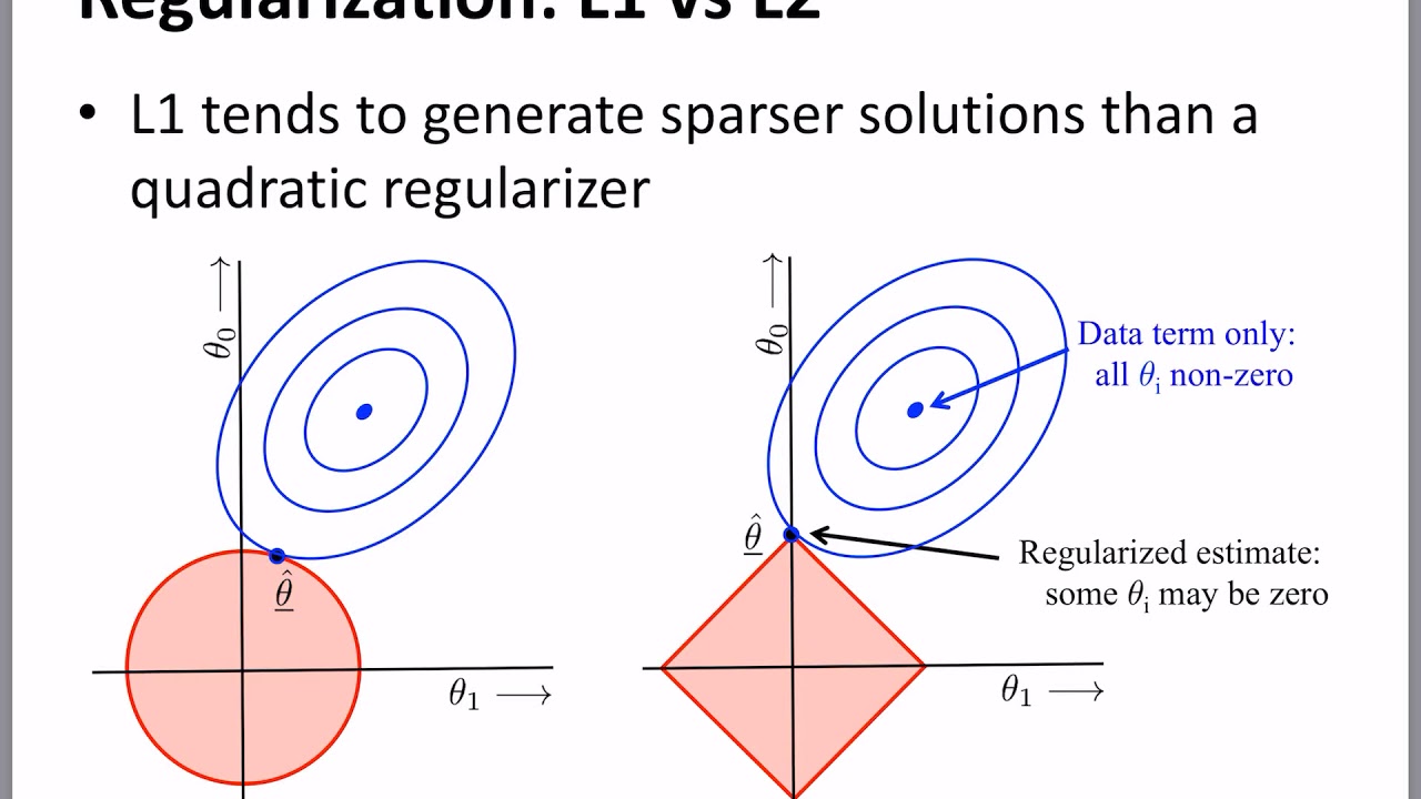
Because L1 can zero out weights, it performs automatic feature selection. If you have many features and suspect some are useless, Lasso can identify and discard them by setting their corresponding weights to zero.

The StatQuest video you saw earlier explains this property very clearly.

Conclusion

In this lesson, you've learned how to implement L1 (Lasso) regularization. While it starts with a simple change to the penalty term, it results in a profoundly different and powerful behavior.

Key Takeaways:

• L1 (Lasso) Regularization adds a penalty to the cost function equal to the sum of the absolute values of the weights, scaled by $\lambda$.
• The gradient of the L1 penalty is constant (except at zero), which gives it a consistent push towards zero during gradient descent.
• This property leads to sparsity, where many model weights become exactly zero.
• Because of sparsity, L1 regularization effectively performs automatic feature selection, making it excellent for models with many potentially irrelevant features.
• The implementation requires handling the non-differentiable nature of the absolute value function, often with a conditional statement or np.sign().

Preview of the Next Lesson:
You have now implemented the core logic for both L1 and L2 regularization. In the next lesson, we will put it all together. You will apply L1 and L2 regularization to the from-scratch Linear and Logistic Regression models you've developed, creating a complete, regularized training pipeline.