Regularization: Preventing Overfitting and Controlling Complexity

1. The Problem of Overfitting: When Models Learn Too Much

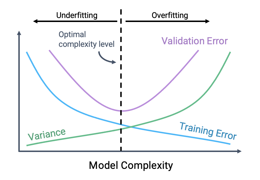
An overfit model is like a student who memorizes the answers to a practice exam but hasn't learned the underlying concepts. They'll ace the practice test, but fail the real one. In machine learning, this means the model performs exceptionally well on the training data but poorly on new, unseen data (like a validation or test set).

The opposite of overfitting is underfitting. An underfit model is too simple to capture the underlying patterns in the data. This would be like trying to fit a straight line to data that follows a curve.

The Bias-Variance Trade-off

The concepts of underfitting and overfitting are formally described by the bias-variance trade-off.

• Bias is the error from erroneous assumptions in the learning algorithm. High bias can cause an algorithm to miss relevant relations between features and target outputs (underfitting). A simple linear model, for instance, has high bias if the true relationship is non-linear.
• Variance is the error from sensitivity to small fluctuations in the training set. High variance can cause an algorithm to model the random noise in the training data, rather than the intended outputs (overfitting).

To get a more intuitive feel for bias and variance, watch the following video from StatQuest.

As the video explains, our goal is to find a model with both low bias and low variance. We want a model that is complex enough to capture the true underlying patterns but not so complex that it models the noise.

2. What is Regularization?

Now that we understand the problem, let's look at the solution. Regularization is a set of techniques used to prevent overfitting by adding a penalty term to the model's loss function.

The standard loss function (like MSE or Cross-Entropy) encourages the model to minimize its prediction error on the training data. The new, regularized loss function looks like this:

$\text{New Loss}=\text{Original Loss}+\lambda \times \text{Regularization Penalty}$

Here, $\lambda$ (lambda, also called alpha in many libraries) is a hyperparameter that controls the strength of the regularization.

The key idea is that the Regularization Penalty is a function of the model's parameters (its weights). This penalty term discourages the model from learning large weights.

Why does this help? A model with large weights is often a complex one. The output of such a model can change drastically with small changes in the input features, leading to the kind of jagged, noise-fitting decision boundaries characteristic of overfitting. By penalizing large weights, we encourage the model to find a simpler solution that generalizes better.

For a deeper dive into this concept, let's turn to a well-written article.

3. How Regularization Affects Model Complexity

The optimization process now faces a trade-off. It wants to minimize the original loss (fit the training data well) but also minimize the regularization penalty (keep the weights small).

• If $\lambda =0$: There is no penalty. The model is free to learn large weights and overfit the training data.
• If $\lambda >0$: The model is punished for having large weights. It must find a balance. It might accept a slightly higher training error in exchange for having smaller weights, which typically leads to a lower error on unseen data.
• If $\lambda \to \infty$: As we discussed, the penalty becomes all-important, and the weights are driven to zero, leading to underfitting.

This trade-off is the essence of how regularization simplifies a model. It pulls the model away from a "perfect" solution that is tailored only to the training set and towards a simpler, more robust solution.

The following article offers several excellent intuitions for why this works.

There are different ways to define the regularization penalty, with the two most common being L1 and L2 regularization.

• L2 Regularization (Ridge): The penalty is the sum of the squared values of the weights. This encourages all weights to be small.
• L1 Regularization (Lasso): The penalty is the sum of the absolute values of the weights. This can push some weights to become exactly zero, effectively performing feature selection.

We will dive deep into the implementation and specific effects of L1 and L2 in the upcoming lessons.

Conclusion

In this lesson, you've built the conceptual foundation for understanding one of the most important techniques for training modern machine learning models.

Key Takeaways:

• Overfitting occurs when a model is too complex, learning the noise in the training data and failing to generalize to new data. This is a state of high variance.
• Model complexity is often associated with large parameter (weight) values.
• Regularization prevents overfitting by adding a penalty for large weights to the loss function.
• This forces the model to find a simpler solution that balances fitting the training data with maintaining small weights, leading to better generalization.
• The strength of regularization is controlled by a hyperparameter, $\lambda$, which must be tuned to find the right balance between underfitting and overfitting.

Preview of the Next Lesson:
With the "why" firmly established, we can now move on to the "how." In the next lesson, you will modify the cost function and its gradient to include an L2 (Ridge) regularization term. We will derive the new gradient update rule and apply it to the regression and classification models you have already built, seeing firsthand how it affects the learning process.