Understanding DFAs: Definition and Tracing

1. The Core Idea: A Machine with Finite Memory

Before diving into formalisms, let's build an intuition for what a finite automaton is. At its core, it's an abstract model of a machine that has a fixed, finite number of "states" or "configurations." It processes an input string of symbols one by one, and each symbol causes the machine to transition from its current state to a new one. The computation is determined entirely by the sequence of states it visits.

A simple light switch is a good analogy. It has two states: On and Off. The inputs are "flick switch up" and "flick switch down." If the light is Off (the state) and you provide the input "flick up," it transitions to the On state. This is the fundamental principle: a current state, an input, and a resulting next state.

To see this idea applied to a computational problem, watch the first part of the following video from MIT OpenCourseWare. It introduces a simple finite automaton and its components using a "state diagram."

As you saw, the machine's "language" is the set of all input strings that it accepts. The example machine, M1, accepts any string of 0s and 1s that contains "11" as a substring. This simple device, with just three states, can solve a specific pattern-matching problem.

2. The Formal Definition of a DFA

Visual diagrams are intuitive, but for rigorous analysis and proofs, we need a precise mathematical definition. This aligns with your preference for starting with abstract principles. A formal definition eliminates ambiguity and allows us to reason about these machines' properties universally.

A Deterministic Finite Automaton (DFA) is formally defined as a 5-tuple (a list of five mathematical objects):
$M=(Q,\Sigma ,\delta ,q_0,F)$
Where:

1. $Q$ is a finite set of states.
2. $\Sigma$ (Sigma) is a finite set called the alphabet, which defines the allowed input symbols.
3. $\delta$ (delta) is the transition function. It dictates the machine's movement. It is a function $\delta :Q\times \Sigma \to Q$, meaning it takes a state from $Q$ and a symbol from $\Sigma$ as input and returns the next state in $Q$. The "deterministic" part of the name comes from the fact that for any given state and input symbol, there is exactly one next state.
4. $q_0\in Q$ is the start state, where the machine begins its computation.
5. $F\subseteq Q$ is the set of accept states (or final states).

To solidify this abstract definition, let's watch the next segment of the MIT video, where Prof. Sipser formalizes the machine M1 from the introduction.

The following image provides another excellent summary, showing a state diagram, its formal 5-tuple definition, and its transition table side-by-side.

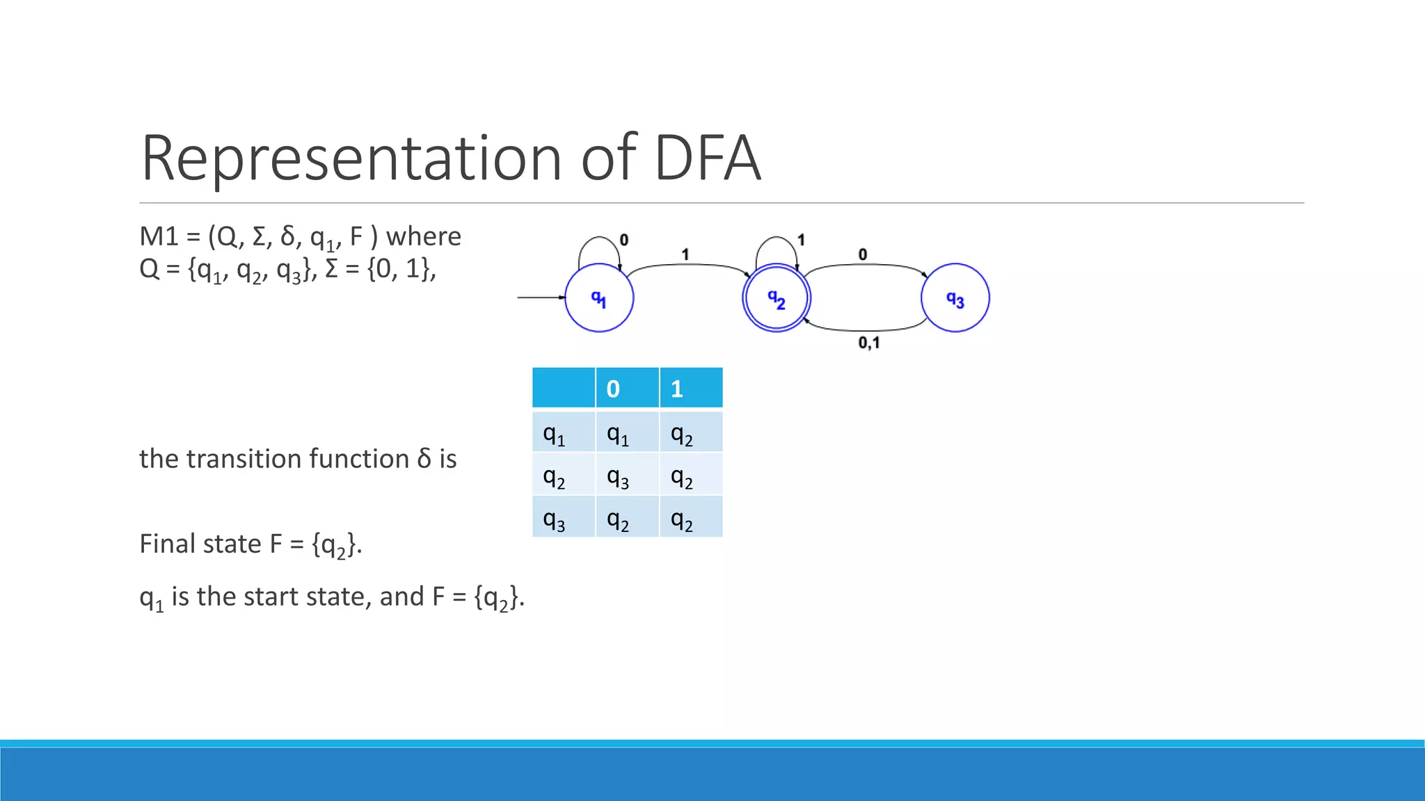
For a concise, text-based reference on these definitions, you can review the following document.

3. Tracing a Computation

Now that we have a formal definition, let's define computation formally. A DFA computes on an input string by processing it one symbol at a time, starting from the start state.

We can trace this process using instantaneous configurations. A configuration is represented as a pair [q, w], where q is the current state and w is the remaining (unread) part of the input string.

A single step of computation is denoted by the ⊢ ("yields") symbol. If the machine is in state $q_i$ with ax as the remaining string (where a is the next symbol and x is the rest of the string), and if $\delta (q_i,a)=q_j$, we write:
$[q_i,ax]⊢[q_j,x]$
This reads: "The configuration [q_i, ax] yields the configuration [q_j, x] in one step."

A full computation is a sequence of such steps. We use ⊢* to denote a sequence of zero or more steps.

A DFA $M=(Q,\Sigma ,\delta ,q_0,F)$ accepts an input string $w$ if the computation starting from the initial configuration $[q_0,w]$ ends in a configuration $[q_f,ϵ]$ where $q_f$ is an accept state ($q_f\in F$). Here, $ϵ$ (epsilon) represents the empty string, signifying that all input has been read. If the final state is not in $F$, the string is rejected.

Let's trace the string ababb on the following machine M1, which is designed to accept any string containing bb.

The formal definition of this machine is:

• $Q=\{0,1,2\}$
• $\Sigma =\{a,b\}$
• $q_0=0$
• $F=\{2\}$
• $\delta$ is given by the diagram.

Trace for input ababb:

1. Start: The initial configuration is [0, ababb].
2. Read 'a': $\delta (0,a)=0$. So, [0, ababb] ⊢ [0, babb].
3. Read 'b': $\delta (0,b)=1$. So, [0, babb] ⊢ [1, abb].
4. Read 'a': $\delta (1,a)=0$. So, [1, abb] ⊢ [0, bb].
5. Read 'b': $\delta (0,b)=1$. So, [0, bb] ⊢ [1, b].
6. Read 'b': $\delta (1,b)=2$. So, [1, b] ⊢ [2, \epsilon].

The computation ends in state 2. Since $2\in F$, the string ababb is accepted.

Trace for input ababa:

1. [0, ababa]
2. ⊢ [0, baba] (reading 'a')
3. ⊢ [1, aba] (reading 'b')
4. ⊢ [0, ba] (reading 'a')
5. ⊢ [1, a] (reading 'b')
6. ⊢ [0, \epsilon] (reading 'a')

The computation ends in state 0. Since $0\notin F$, the string ababa is rejected.

Your Turn: Practice Tracing

Now, use the DFA pictured below, which is designed to accept strings with an even number of 0s. The start state is $q_0$, which is also the only accept state.

Trace the computation for the input string 1011001. Does the machine accept or reject this string? Write down the sequence of configurations.

Conclusion

In this lesson, we established the first building block in our study of computation. We explored the intuitive concept of a finite automaton and, more importantly, solidified it with a precise, formal definition.

Here are the key takeaways:

• A Deterministic Finite Automaton (DFA) is a model of a machine with finite memory, represented formally as a 5-tuple: $M=(Q,\Sigma ,\delta ,q_0,F)$.
• The machine's behavior is dictated by the transition function $\delta$, which deterministically maps a current state and an input symbol to a single next state.
• A DFA computes by reading an input string symbol by symbol, transitioning between states. We can formally track this process using instantaneous configurations.
• A string is accepted if the machine ends in a state belonging to the set of accept states $F$. Otherwise, it is rejected.
• The set of all strings a machine $M$ accepts is called the language of the machine, denoted $L(M)$.

While simple, DFAs are powerful enough to form the basis for practical tools like text search utilities (e.g., grep), network packet filters, and the lexical analyzers in compilers that tokenize source code.

In our next lesson, we will introduce a seemingly more powerful type of finite automaton: the Nondeterministic Finite Automaton (NFA). NFAs can have multiple possible next states for a single input, introducing an element of "choice." This will lead us to a fundamental question: does this added flexibility of nondeterminism allow these machines to recognize languages that DFAs cannot?