NFA: Definition and Tracing Computation

In our previous lesson, we established a rigorous foundation for the most basic model of computation, the Deterministic Finite Automaton (DFA). The key feature of a DFA is its predictability: for any given state and input symbol, there is exactly one next state. Today, we will explore what happens when we relax this rigid constraint by introducing nondeterminism.

This lesson introduces the Nondeterministic Finite Automaton (NFA). You will learn its formal definition and, crucially, how to trace the computation of an input string when multiple paths—or no paths—are possible. This new model will seem more flexible and powerful than a DFA, which sets the stage for a fundamental question we will tackle in our next lesson: Does this added flexibility actually increase the computational power of these machines?

1. The Idea of Nondeterminism

In a DFA, the machine's path is uniquely determined by the input string. An NFA introduces three new capabilities that break this determinism:

A state may have multiple transitions for a single input symbol.
A state may have zero transitions for a single input symbol, causing that path of computation to "die."
A state may have transitions on the empty string $ϵ$ , allowing the machine to change state without consuming any input.

These features mean that from a given state and on a given input symbol, the machine could transition to a set of possible next states. To see this in action, let's turn again to Prof. Sipser's lecture from MIT OpenCourseWare.

2. Nondeterminism, Closure Properties, Conversion of Regular Expressions to FA

This video will introduce the core concepts of nondeterminism by contrasting an NFA directly with the DFAs we've already seen.

Watch from the introduction to nondeterminism. Pay close attention to the example NFA he presents and the two key differences he highlights: multiple transitions for the same symbol and \epsilon-transitions.

2. Formal Definition of an NFA

As you prefer to work from abstract principles, let's formalize this new model. Like a DFA, an NFA is a 5-tuple, but with a critical modification to the transition function.

A Nondeterministic Finite Automaton (NFA) is a 5-tuple $N = (Q, Σ, δ, q_{0}, F)$ , where:

$Q$ is a finite set of states.
$Σ$ is a finite alphabet.
$δ$ is the transition function. This is the main difference. The function is $δ : Q \times (Σ \cup {ϵ}) \to P (Q)$ .
- The domain $Q \times (Σ \cup {ϵ})$ shows that the function takes a state and either an alphabet symbol or the empty string $ϵ$ as input.
- The codomain $P (Q)$ is the power set of $Q$ . The power set is the set of all subsets of $Q$ . This means the function returns a set of possible next states.
$q_{0} \in Q$ is the start state.
$F \subseteq Q$ is the set of accept states.

The image below gives a clear example, connecting the formal 5-tuple, a state diagram, and the transition table. Notice how $δ (q_{0}, a)$ maps to the set ${q_{0}, q_{1}}$ and how the transition on $ϵ$ is handled.

Caption: An example of a Nondeterministic Finite Automaton (NFA) showing its formal 5-tuple definition, a state diagram, and a transition table. This illustrates how the transition function $\delta$ maps to a set of states, the core feature of nondeterminism.

To deepen your understanding of the transition function mapping to a power set, the following reading provides a very clear, formal definition.

Nondeterministic Finite Automata

These lecture notes from the University of Illinois provide a rigorous and well-structured definition of an NFA.

Read section "1.1 Nondeterministic Finite Automata (NFA)". Focus on Definition 1 and how it formally captures the features of multiple transitions and \epsilon-transitions through the domain and codomain of \delta. Compare the formal description of the example NFA with its diagram in Figure 1.

3. Tracing an NFA Computation

Since an NFA can follow many different computational paths for a single input, how do we determine acceptance? The rule is simple:

An NFA accepts an input string if at least one of the possible computation paths ends in an accept state.

To trace a computation, we can't track a single current state like we did with DFAs. Instead, we must track the set of all possible current states as the machine reads the input.

Let's say the machine is currently in a set of active states $S$ . When the next input symbol $a$ is read, the new set of active states $S^{'}$ is found by:

For each state $q \in S$ , find the set of states reachable from $q$ on input $a$ . This is given by $δ (q, a)$ .
Take the union of all these resulting sets.
Crucially, we must also account for $ϵ$ -transitions. The final set of active states includes all states reachable from $S^{'}$ by following any number of $ϵ$ -transitions. This is often called the $ϵ$ -closure.

After the entire string is read, if the final set of active states contains at least one accept state (i.e., its intersection with $F$ is non-empty), the string is accepted.

The following video provides an excellent, step-by-step trace of several input strings.

2. Nondeterminism, Closure Properties, Conversion of Regular Expressions to FA

Watching Prof. Sipser trace computations will solidify your understanding of how to manage the set of active states.

First, watch from the acceptance rule, where he explains how acceptance works and traces the input a b. Then, continue from more examples to see how other strings like a a, a b a, and a b b are processed, including cases where computation paths "die."

The process of an NFA computation can be visualized as a tree of possibilities, where each branch represents a different computational path. The input string is accepted if any branch ends in an accepting state.

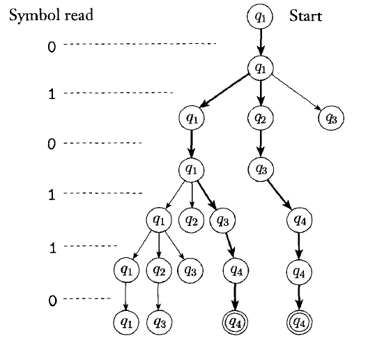
Caption: A tree diagram illustrating the computation of an NFA. Each level shows the set of active states after reading an input symbol. The input is accepted because at least one path (the leftmost branch) terminates in an accept state (q4).

4. Three Views of Nondeterminism

The formal mechanism of tracking sets of states is precise, but there are more intuitive, and philosophically interesting, ways to think about what nondeterminism means. These perspectives will be very useful as we encounter more complex computational models.

Parallel Computation: Think of the NFA as forking into multiple copies of itself at each choice point. Each copy runs in parallel, exploring one possible path. If any copy is in an accept state after reading the input, the original machine accepts.
Tree of Possibilities: This is the view shown in the image above. The computation is a tree where nodes represent states and edges represent transitions. The root is the start state. The string is accepted if any path from the root to a leaf node (after reading the whole string) ends in an accept state.
Magical Guessing: This is a powerful abstraction. Imagine the NFA is endowed with a "perfect guesser" or an oracle. At every point where there is a choice of transition, it magically guesses the correct one—that is, the one that will lead to an accepting state, if such a path exists. If no accepting path is possible, it doesn't matter what it guesses; the string will be rejected. This view recasts the problem from exploring all paths to simply verifying if a "good" path exists.

The following short video segment discusses these three perspectives.

2. Nondeterminism, Closure Properties, Conversion of Regular Expressions to FA

This part of the lecture connects the technical process to higher-level concepts.

Watch the segment on the intuitive understanding of nondeterminism from the three views. The "magical guessing" view, in particular, will be a recurring theme in complexity theory.

Your Turn: Practice Tracing

Let's apply what you've learned. Consider the following NFA, which is designed to accept any string over ${0, 1}$ that ends with 01.

Caption: An NFA that accepts strings ending in 01. State q0 is the start state, and q2 is the accept state.

Trace the computation for the input string 1001. What is the set of active states after each symbol is read? Does the machine accept or reject the string?

Solution

Let's trace the computation for the input string 1001. We'll keep track of the set of active states.

Initial state: Before reading any input, the machine is only in the start state.
- Active states: ${q_{0}}$
After reading '1': From $q_{0}$ , there is a transition on '1' back to $q_{0}$ .
- Active states: ${q_{0}}$
After reading '0' (the second symbol): From $q_{0}$ , a '0' can lead to $q_{0}$ (loop) or to $q_{1}$ . So the machine is now in two states simultaneously.
- Active states: ${q_{0}, q_{1}}$
After reading '0' (the third symbol): We check transitions for each active state:
- From $q_{0}$ on '0': go to ${q_{0}, q_{1}}$ .
- From $q_{1}$ on '0': there is no transition, so this path dies.
- The union of the results is ${q_{0}, q_{1}}$ .
- Active states: ${q_{0}, q_{1}}$
After reading '1' (the final symbol): We check transitions for each active state:
- From $q_{0}$ on '1': go to ${q_{0}}$ .
- From $q_{1}$ on '1': go to ${q_{2}}$ .
- The union of the results is ${q_{0}, q_{2}}$ .
- Final active states: ${q_{0}, q_{2}}$

The entire string has been read. The final set of active states is ${q_{0}, q_{2}}$ . We check if this set contains any accept states. Since $q_{2}$ is an accept state and $q_{2} \in {q_{0}, q_{2}}$ , the string 1001 is accepted.

Conclusion

In this lesson, we expanded our computational toolkit by introducing nondeterminism. We have seen how this new feature changes both the formal definition of a finite automaton and the process of tracing its computation.

Key takeaways from this lesson:

A Nondeterministic Finite Automaton (NFA) allows for multiple next states, zero next states, or transitions on the empty string $ϵ$ .
Formally, this is captured by a transition function $δ$ that maps to the power set of states: $δ : Q \times (Σ \cup {ϵ}) \to P (Q)$ .
An NFA accepts a string if any possible computational path ends in an accept state.
Tracing an NFA involves tracking the set of all active states at each step of the computation.
Nondeterminism can be intuitively understood as parallel computation, exploring a tree of possibilities, or making magical guesses.

NFAs often allow for much simpler and more intuitive designs for recognizing languages compared to DFAs. But does their flexibility grant them superior computational power? Can they recognize languages that DFAs cannot? We will definitively answer this question in the next lesson by proving that NFAs and DFAs are, in fact, equivalent in power. We will do this by introducing an algorithm called subset construction to convert any NFA into an equivalent DFA.

Recommended resources

1. The Idea of Nondeterminism

2. Formal Definition of an NFA

3. Tracing an NFA Computation

4. Three Views of Nondeterminism

Your Turn: Practice Tracing

Conclusion