Hello! Welcome back to our module on Applied Spatial Analysis with GIS.
In our last lesson, we learned how to ask questions of our data using attribute and spatial queries. We saw how a "select by location" query could find features within a certain distance of other features. Today, we will take that concept a step further. Instead of just selecting features, we will learn how to create a new geographic layer that represents this "zone of proximity."
Our learning outcome for this lesson is to apply proximity analysis (buffering) to solve basic spatial problems. By the end of this lesson, you'll understand one of the most common and powerful tools in all of GIS, used in everything from urban planning and environmental protection to business analysis.
1. What is a Buffer?
A buffer is a zone of a specified distance created around a GIS feature. Think of it as drawing a circle around a point, a corridor along a line, or an expanded/shrunken area around a polygon. The core purpose of buffering is to identify areas that are "near" a feature.
This simple idea is incredibly versatile. For example, we can use buffers to answer questions like:
- Which houses are within 500 meters of a proposed new highway?
- What areas of a forest fall within a 1-kilometer radius of a water source?
- Which properties are within the 100-meter "no construction" zone along a riverbank?
To get a solid grasp of the fundamentals, please read the following introductory material.
10. Vector Spatial Analysis (Buffers)
The QGIS documentation provides a clear and concise introduction to buffering. It explains what a buffer zone is and shows how it applies to different vector types (points, lines, and polygons).
Please read the sections '10.1. Overview' and '10.2. Buffering in detail'. Focus on understanding the definition of a buffer zone and recognizing that the output of a buffer operation is always a vector polygon.
As the reading highlights, regardless of whether your input is a point, line, or polygon, the resulting buffer is always a new polygon layer. This new layer can then be used for visualization or further analysis.
2. Types and Variations of Buffers
Not all buffers are the same. GIS software provides several options that allow you to tailor the analysis to your specific problem.
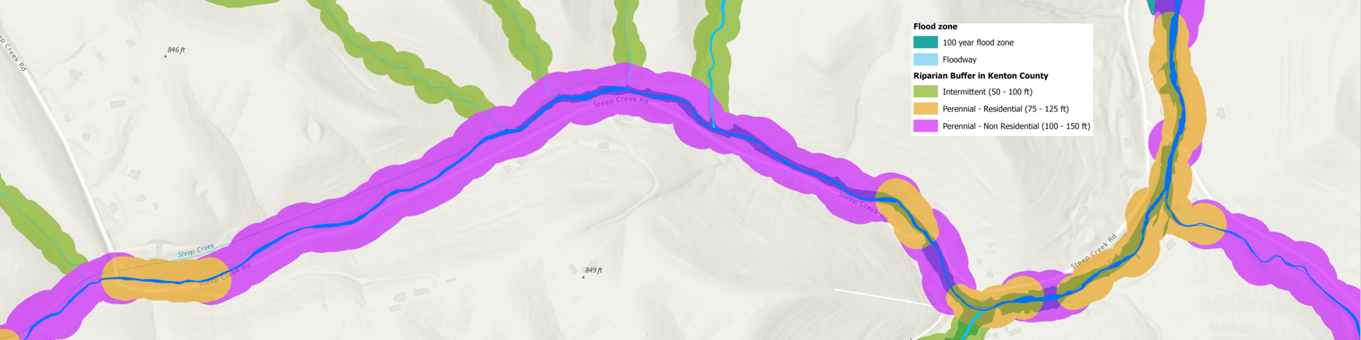
Uniform vs. Variable Buffers
- A uniform buffer applies the same distance to all features in a layer (e.g., a 1km buffer around all schools).
- A variable buffer uses different distances for different features, based on a value in their attribute table. For example, major rivers could have a 100-meter buffer, while minor streams have a 30-meter buffer.
Dissolved vs. Undissolved Buffers
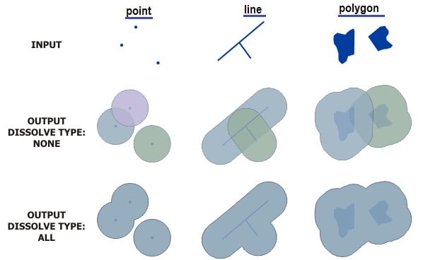
This is a critical concept. When buffers from multiple features overlap, you can choose whether to merge them or keep them as separate, overlapping polygons.
- Dissolved: Overlapping areas are merged into a single, continuous polygon. This is useful when you only care about the total area covered by the buffer.
- Undissolved (or Intact): Each buffer is kept as a separate feature, even if it overlaps with others.
Other Variations
GIS tools also allow for:
- Multiple Ring Buffers: Creating several concentric zones at different distances (e.g., 1km, 2km, and 5km zones around a city).
- Inward Buffers (Setbacks): For polygon features, you can create a buffer on the inside, effectively shrinking the polygon. This is often used for defining construction setbacks from a property line.
This next reading provides more detail and examples for these variations.
The article 'Buffers in GIS' by Geography Realm expands on the different types of buffers and their uses.
Read the sections 'Buffers and GIS data types', 'Variable buffer', and 'Buffer direction in GIS for polygons'. This will reinforce the concepts of uniform, variable, and setback buffers.
3. Applying Buffers to Solve a Spatial Problem
Knowing what a buffer is becomes truly useful when you apply it. The most common workflow involves two main steps:
- Create a buffer around a set of features to define a proximity zone.
- Use that buffer layer in a spatial query (as we learned in the last lesson) to select other features that fall within it.
The following video demonstrates this entire workflow using a practical environmental health scenario: identifying hospitals that might be at risk due to their proximity to solid waste sites.
Buffer Analysis in GIS: Proximity of Hospitals to Solid Waste Sites
This detailed tutorial, 'Buffer Analysis in GIS', walks through a complete spatial problem. It shows not just how to create buffers, but how to use them to derive meaningful results.
Please watch the following segments carefully, paying attention to the two-step analysis process: Step 1: Creating the Proximity Zones (01:16 - 06:18): Watch how the presenter uses the 'Multiple Ring Buffer' tool to create 1, 1.5, and 2-mile zones around the solid waste sites. Notice the use of the 'Dissolve' option. Step 2: Selecting Features within the Zones (09:11 - 12:07): This is the crucial link to our previous lesson. See how the presenter uses 'Select by Location' to find the hospitals that are within the newly created buffer polygons. Step 3: Classifying the Results (12:07 - 17:55): Observe how the selected hospitals are exported into new layers (high-risk, medium-risk, etc.) to create a final, informative map.
The video uses ArcGIS, a popular commercial GIS software. The same principles apply to all GIS platforms, including the free and open-source QGIS. The following short video shows how the buffer tool works in QGIS and gives another clear explanation of the "dissolve" option.
To see these concepts in another environment, the video 'How to buffer things in QGIS' provides a quick and clear demonstration.
Watch from the beginning until 02:13. The key takeaway is seeing how an undissolved buffer on a segmented line looks messy, and how checking the 'dissolve result' box cleans it up into a single, useful polygon.
Test your understanding!
A city wants to enforce a new law stating that no new fast-food restaurants can open within 300 meters of any school. You have been given two GIS layers:
- A point layer of all
Schools. - A point layer of all
Proposed_Restaurants.
Describe the two main steps you would take in a GIS to identify which of the proposed restaurants violate the new law.
Show answer
-
Step 1: Create the Proximity Zone. You would use the buffer tool on the
Schoolslayer to create a new polygon layer. The buffer distance would be set to 300 meters. You would likely use the "dissolve" option to merge any overlapping zones into a single restricted area. -
Step 2: Select the Violating Restaurants. You would then perform a spatial query ("Select by Location"). You would select features from the
Proposed_Restaurantslayer that are within (or intersect) the new 300-meter buffer layer you created in the first step. The selected points would be the restaurants that violate the law.
Conclusion
Today you've learned how to perform proximity analysis, one of the cornerstones of GIS. By creating buffers, you can move beyond simple selection and generate new data that explicitly represents nearness. This ability to define and analyze spatial relationships is what makes GIS such a powerful tool for understanding our world.
Key Takeaways:
- Buffering is a proximity analysis tool that creates a polygon zone of a specified distance around features.
- The output of a buffer operation is always a new polygon layer.
- Important buffer variations include uniform vs. variable distance, and dissolved vs. undissolved boundaries.
- A common and powerful workflow is to first create a buffer, and then use that buffer in a spatial query to select features from another layer.
Preview of the Next Lesson:
We've now seen how to create a new layer based on proximity. In our next lesson, we will explore overlay analysis. Overlay allows you to combine two or more layers to create a new output layer that contains information from all of them. For instance, you could overlay a buffer layer with a land-use layer to calculate exactly how many acres of wetland fall within a proposed development's impact zone. This will open up an even wider range of analytical possibilities.