Hello! Welcome to the third lesson in our module on Applied Spatial Analysis.
In our last session, we explored proximity analysis by creating buffers—new polygon layers representing a zone of a specified distance around features. We saw how this could define, for example, a 300-meter "exclusion zone" around schools. But what do we do with that new layer? How do we combine it with other data, like a layer of proposed restaurants, to get a final answer? That is the focus of today's lesson.
Our learning outcome is to use overlay analysis to integrate multiple data layers for relationship analysis. This is one of the most powerful and fundamental capabilities in all of GIS. By the end of this lesson, you will understand how to combine different spatial datasets to create new, synthesized information that answers complex questions.
1. What is Overlay Analysis?
At its core, overlay analysis involves "stacking" multiple map layers on top of each other to analyze the relationships between their features. Imagine placing several transparent maps on a light table; the patterns you see in the combined view reveal new insights.
This idea predates computers. In the 1850s, Dr. John Snow famously overlaid a map of cholera deaths with a map of water pump locations in London to pinpoint the source of the outbreak. This was a manual form of overlay analysis. Today, GIS provides powerful digital tools to perform these operations with precision and speed.
To get a formal introduction to this concept, please read the first section of the following text.
The following reading from 'GIS Commons' introduces the core concept of overlay analysis and its historical roots.
Read the introductory section, starting from 'Overlay is one of the most common and powerful GIS functions' and ending just before the heading 'Vector (Logical) Overlay'. Focus on understanding the general purpose of overlay.
GIS performs overlay analysis on both vector and raster data, but the methods differ. In this lesson, we will focus primarily on vector overlay, as it builds directly on our previous work with points, lines, and polygons.
2. The Tools of Vector Overlay
Vector overlay combines the geometries and attributes of two input layers to create a new output layer. The most common overlay operations are based on logical operators like AND, OR, and NOT.
To see how these work in practice, let's watch a short video that demonstrates the main vector overlay tools in a GIS.
GIS vector overlay tools: clip, intersection, union, (symmetrical) difference
This video by Hans van der Kwast provides a concise and clear demonstration of the four most common vector overlay tools: Clip, Difference, Intersect, and Union.
Watch the entire video (it's about 4.5 minutes long). For each tool, pay close attention to two things: What happens to the geometry (the shapes)? What happens to the attributes (the data in the table)?
Let's summarize what you just saw. These operations are the building blocks of most vector-based spatial analysis.
- Intersect (AND): This tool creates a new layer containing only the areas where the two input layers overlap. The new features will have the attributes from both input layers. This is useful for finding locations that meet two criteria simultaneously (e.g., areas that are both residential zones AND within a floodplain).
- Union (OR): This tool combines all features from both input layers into a single new layer. It preserves all geometries from both layers and their attributes. Where features overlap, the attributes are combined. This is useful for creating a composite layer from two separate datasets (e.g., combining a layer of wetlands with a layer of forests to create a single 'natural areas' map).
- Clip: This tool acts like a cookie cutter. It uses the geometry of one layer (the "clip layer") to cut out a piece of another layer (the "input layer"). The output contains only the part of the input layer that was inside the clip layer, and it only retains the attributes of the input layer. This is useful for trimming a large dataset down to your specific area of interest.
- Difference (NOT): This tool subtracts the geometry of one layer from another. It keeps the parts of the input layer that do not overlap with the "difference layer". Think of it as erasing one feature with another.

Test your understanding!
You are an environmental analyst with two vector layers:
- A polygon layer showing
Protected_Forests. - A polygon layer showing the path of a
Proposed_Highway.
Which overlay tool would you use to create a new layer that shows exactly which parts of the protected forests would be destroyed by the highway's construction?
Show answer
The best tool for this is Intersect. By intersecting the Protected_Forests layer with the Proposed_Highway layer, the output will be a new polygon layer representing only the areas where the two overlap. This new layer precisely delineates the conflict zones and would allow you to calculate the exact area of forest that is at risk.
3. A Strategy for Overlay: Suitability Modeling
Knowing how the tools work is the first step. The next is knowing how to combine them to solve a complex problem. One of the most common applications of overlay analysis is suitability modeling—the process of finding the best locations for a particular purpose.
This involves defining a set of criteria, creating a map layer for each criterion, and then combining them to find the locations that meet all (or most) of the criteria. This requires a systematic approach.
Understanding overlay analysis
The documentation for ArcGIS Pro outlines a general, step-by-step methodology for performing overlay analysis. While the software is different, the strategic thinking applies to any GIS platform.
Please read from the beginning down to the end of step '1. Define the problem'. Focus on understanding the overall purpose of suitability modeling and the importance of clearly defining the problem you are trying to solve.
As the reading describes, a typical workflow for a suitability model involves these general steps:
- Define the problem: What are you trying to find? (e.g., "the best location for a new park").
- Determine significant layers (criteria): What factors are important? (e.g., must be on city-owned land, must not be on a steep slope, should be far from existing parks).
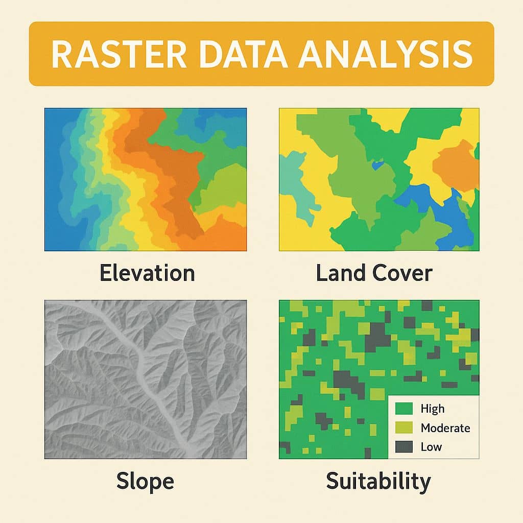
- Reclassify/Transform: Often, you need to process your input layers to make them comparable. For raster overlay, this involves putting all data on a common scale (e.g., 1-10). For vector, it might involve creating buffers or selecting certain features.
- Combine the layers: Use overlay tools like Intersect, Union, and Difference to combine your criteria layers and find the locations that satisfy your rules.
- Analyze the results: Examine the final locations to see if they make sense.
This process allows us to combine layers representing very different things—like slope, land ownership, and proximity—into a single, analytical framework.
4. Case Study: Finding Suitable Bicycle Parking Locations
Now, let's put everything together and see how this strategic process works in a real-world scenario. The following video demonstrates a multi-criteria overlay analysis in QGIS to find the best locations for new bicycle parking facilities in London.
This example is powerful because it combines:
- Proximity analysis (buffering from our last lesson).
- Overlay analysis (Intersect and Difference).
- A clear, structured problem-solving approach.
Multiple Criteria Overlay Analysis Using QGIS (Vector Data)
This video from Geo Guru walks through a complete multi-criteria overlay analysis to solve a real-world problem.
Watch from the beginning to 08:06. As you watch, try to map the presenter's actions to the strategic steps we just discussed: Defining the Problem & Criteria (00:01 - 01:18): Listen for the three criteria for a suitable site. Preparing the Layers (01:18 - 06:06): Notice how they prepare the layers for each criterion. This includes converting a raster heat map to a vector polygon and creating buffers (just like we did in the last lesson!). Combining Layers (06:06 - 08:06): Observe how they first use Intersection to find areas that meet the first two (inclusive) criteria, and then use Difference to apply the final (exclusive) criterion.
This case study is a perfect example of the lesson's learning outcome. It shows how multiple layers (theft hotspots, cycle routes, existing parking) are integrated using overlay tools to perform a relationship analysis, resulting in a new layer of suitable locations.
Conclusion
Today, we have unlocked one of the most essential analytical functions in GIS. Overlay analysis moves beyond looking at single layers and allows us to create new knowledge by combining them. You've seen that this process involves both understanding the mechanics of tools like Intersect and Union, and applying them within a structured, strategic framework to solve complex spatial problems like site selection.
Key Takeaways:
- Overlay Analysis is the process of combining two or more spatial layers to create a new output layer that synthesizes their information.
- The primary vector overlay tools are Intersect (AND), Union (OR), Clip, and Difference (NOT), each serving a different logical function.
- A common application of overlay is suitability modeling, a systematic process for finding the best locations that meet a set of criteria.
- A typical workflow involves defining the problem, preparing layers for each criterion (e.g., through buffering or selection), and then combining them using overlay tools to find a solution.
Preview of the Next Lesson:
In this lesson and the previous one, our focus has been primarily on vector analysis tools. For our next topic, we will shift our attention back to raster data. We will explore how to generate and interpret terrain analysis outputs like slope, aspect, and hillshade from a Digital Elevation Model (DEM). This will open up a new set of capabilities for understanding and visualizing the Earth's surface.