GIS for Environmental Analysis

1. The GIS Project Framework

Every rigorous GIS analysis follows a structured process, from defining the problem to presenting the results. This systematic approach ensures the analysis is logical, repeatable, and clearly understood. For our case study, we'll follow these general steps:

1. State the Problem: Identify areas at high risk of flooding within a specific geographic region.
2. Acquire Data: Gather the necessary spatial data representing the key factors that contribute to flood risk.
3. Process and Prepare Data: Use GIS tools to derive new datasets from our initial data (e.g., creating a slope map from an elevation model).
4. Analyze the Data: Combine the various data layers using a structured methodology to calculate a final risk score.
5. Visualize and Interpret Results: Create a final map that clearly communicates the areas of low, medium, and high risk.

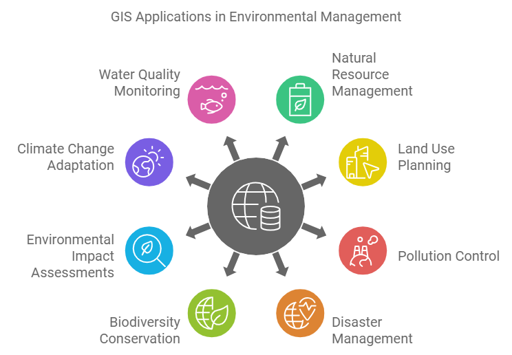
The core of our analysis will be a method called Multi-Criteria Evaluation (MCE). MCE is a powerful decision-making technique used in GIS to evaluate scenarios based on multiple factors. We will identify the key physical geography factors contributing to flood risk, create a data layer for each, and then combine them to produce a final flood risk map.

For our flood risk model, we will use five key factors, based on common hydrological practice:

• Elevation: Lower-lying areas are more susceptible to flooding.
• Slope: Flatter areas allow water to accumulate rather than drain away quickly.
• Precipitation: Areas with higher rainfall are more likely to experience flooding.
• Land Cover: The type of surface (e.g., forest, pavement, wetland) affects how much water is absorbed versus how much runs off.
• Proximity to Streams: Areas closer to existing rivers and streams are at a higher risk of inundation.

2. A Complete Walkthrough: Flood Risk Mapping

To guide us through this entire process, we will use a detailed video tutorial. While the video uses ArcGIS, the principles, tools, and workflow are conceptually identical to what you would do in QGIS or other professional GIS software.

3. Part 1: Data Acquisition and Preparation

First, we need to gather and create the five data layers for our model.

Elevation and Slope

You are already familiar with Digital Elevation Models (DEMs) and how to derive a slope map from one. In our case study, the DEM and slope map are considered our starting data.

Precipitation Data

Climate data is a crucial input. The video demonstrates a standard method for obtaining global precipitation data.

Deriving the Stream Network

Just as in our last lesson, the stream network isn't raw data; it's derived from the DEM. This part of the tutorial is an excellent practical review of the watershed delineation workflow.

Calculating Proximity to Streams

Now that we have a stream network, we can calculate our final input factor: the distance of every location from the nearest stream.

At this point, we have all five of our input layers ready for analysis.

4. Part 2: The Core Analysis - Reclassification

This is the most important conceptual step in our MCE. We cannot directly combine elevation (in meters), slope (in degrees), and precipitation (in millimeters). The units and value ranges are incompatible. We must first standardize all layers by reclassifying them onto a common, unitless scale that represents flood risk.

The video uses a simple 1-to-10 scale, where a higher score means higher flood risk.

This process of reclassification transforms our raw physical data into five separate layers, each representing a different facet of flood risk.

5. Part 3: Combining Layers and Interpreting the Result

With all our factors reclassified to the same risk scale, we can finally combine them. However, not all factors are equally important. For instance, being 1 meter away from a river might be a more significant risk factor than having a very gentle slope. We account for this using a Weighted Sum.

In a weighted sum (or weighted overlay), each reclassified risk layer is multiplied by a weight (a percentage) that reflects its importance in the overall model. The final risk score for each cell is the sum of all its weighted risk scores.

The choice of weights is critical and is usually based on expert knowledge, local conditions, or statistical analysis. Different weights will produce different results.

Finally, the raw output of the weighted sum is a continuous raster of risk scores. For easier interpretation, it's common to classify this final map into categories like 'Very Low Risk', 'Low Risk', 'Medium Risk', 'High Risk', and 'Very High Risk', as shown in the final part of the video (00:39:53 - 00:41:52).

6. The Bigger Picture: From Analysis to Action

The flood risk map you have just learned to create is not just an academic exercise. It is a powerful tool for real-world planning and climate resilience. To understand how this kind of analysis fits into a broader context, let's briefly look at a conceptual framework.

This shows that the map we create is a crucial input for helping planners identify where to invest in flood defenses, update zoning regulations, or develop emergency response plans.

Conclusion

Congratulations on completing the final lesson and the entire course! You have successfully integrated knowledge from physical geography and practical skills in GIS to conduct a complete environmental analysis.

Key Takeaways:

• Multi-Criteria Evaluation (MCE) is a standard GIS methodology for analyzing complex problems by combining multiple data layers.
• A successful MCE requires a clear framework: defining the problem, selecting relevant criteria (factors), and acquiring the data.
• Reclassification is the essential step of standardizing all input layers to a common, unitless scale (e.g., a risk score) before they can be combined.
• A Weighted Sum is used to combine the reclassified layers, assigning more importance to more influential factors.
• The entire process, from data acquisition to final map, represents a geospatial model—a simplified representation of a real-world environmental process.
• The outputs of these models are not just maps, but critical inputs for environmental management, planning, and policy-making.

You began this course as a beginner and have systematically built a strong, foundational understanding of physical geography and the analytical tools used to study it. You are now equipped with the concepts and skills to explore the world through a geographic lens, to ask spatial questions, and to understand the methods used to answer them. Well done