Hello! Welcome to the sixth lesson in our module on Applied Spatial Analysis with GIS.
In our last lesson, we focused on deriving fundamental terrain attributes from a Digital Elevation Model (DEM). You learned how to generate and interpret slope, aspect, and hillshade maps, transforming a raw elevation dataset into layers that describe the steepness, orientation, and visual form of the landscape.
Today, we will build directly on that foundation to tackle one of the most common and powerful applications in physical geography and hydrology. Our learning outcome is to apply GIS tools to a practical problem: delineating a watershed from a DEM. This multi-step process is a perfect example of how the basic analytical components we've learned can be chained together in a logical workflow to solve a complex spatial problem. For you, with your interest in climatology and physical geography, understanding how water flows across a landscape is a foundational skill.
1. Understanding the Goal: What is a Watershed?
Before we dive into the "how," let's clarify the "what." A watershed, also known as a drainage basin or catchment, is an area of land where all precipitation that falls on it drains to a common outlet, such as a point on a river, a lake, or the sea. Delineating a watershed means identifying its precise boundary.
This process is crucial for countless environmental applications, including:
- Flood prediction and mitigation.
- Water quality assessment (e.g., identifying sources of pollution upstream).
- Water resource management.
- Ecological studies of aquatic habitats.
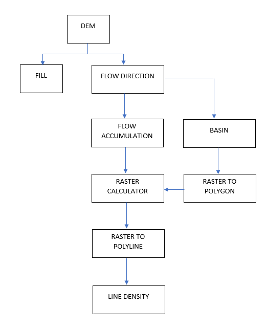
The entire process follows a clear, logical sequence. This flowchart illustrates the typical steps involved.
2. The Conceptual Workflow of Watershed Delineation
While different GIS software might have tools with slightly different names, the underlying hydrological logic is universal. Let's walk through the sequence conceptually.
- Start with a DEM: Our base data is the Digital Elevation Model, which provides the elevation for every cell in our study area.
- Fill Sinks: Raw DEMs often have small imperfections—pixels or groups of pixels with a lower elevation than all their neighbors. These "sinks" would incorrectly trap water in a computer model. The first step is to run a 'Fill' tool to create a "hydrologically corrected" DEM where water can flow continuously downhill.
- Calculate Flow Direction: Using the filled DEM, the GIS calculates the direction of water flow for each cell. The most common method, called D8 (Deterministic 8), assumes water flows from a cell to whichever of its eight neighbors is at the steepest downward slope. The output is a raster where each cell's value represents a direction (e.g., 1=East, 2=Southeast, etc.).
- Calculate Flow Accumulation: This is a key step. The GIS uses the flow direction raster to calculate, for every single cell, how many upstream cells flow into it. Cells with a high flow accumulation value represent areas of concentrated flow—in other words, streams and rivers. The output is a raster where bright lines emerge, tracing the drainage network.
- Define a Pour Point (Outlet): A watershed is always defined relative to a single outlet point. We must manually specify this "pour point" on the stream network. All water from the watershed will exit through this point.
- Delineate the Watershed: Finally, using the flow direction raster and the pour point, the GIS identifies every single cell that flows into that outlet. The collection of all these upstream cells forms the watershed.
Now, let's see how this conceptual workflow is implemented in practice using QGIS.
3. A Practical Guide to Watershed Delineation in QGIS
The most effective way to learn this process is to see it in action. We will be using a comprehensive video tutorial as our main guide. It uses the powerful open-source SAGA tools, which are integrated within QGIS.
Complete QGIS Watershed Delineation Tutorial
The following video from GeoDelta Labs, titled 'Complete QGIS Watershed Delineation Tutorial', provides a complete, step-by-step walkthrough of this entire process. We will break it down into logical segments.
You do not need to watch the video all at once. We will go through it section by section.
Step 1: Data Preparation
Any good GIS analysis begins with preparing your data. This involves ensuring your data is in the correct format and coordinate system for the analysis you want to perform.
Complete QGIS Watershed Delineation Tutorial
Watch the first part of the tutorial, which covers the essential preparatory steps.
Please watch from the beginning (00:00:00) until 16:34. Focus on these key actions: Reprojecting the DEM: Note why the presenter changes the Coordinate Reference System (CRS) from a geographic one (like WGS84, with units in degrees) to a projected one (like UTM, with units in meters). This is crucial for accurate distance and area calculations. Clipping the DEM: Observe how the DEM is clipped to a smaller area of interest. This makes subsequent analysis much faster by reducing the amount of data the computer has to process.
These initial steps of reprojecting and clipping are fundamental best practices for almost any raster analysis project in GIS.
Step 2: Hydrological Correction and Stream Network Generation
Now we move into the core hydrological analysis, starting with creating a valid surface and identifying the river channels.
Complete QGIS Watershed Delineation Tutorial
This next segment covers the first major steps of the hydrological modeling: filling sinks and generating the stream network.
Please watch from 16:34 to 34:18. The video covers three main tools: Fill Sinks (Wang & Liu) (starts at 17:55): This is the practical implementation of creating a hydrologically corrected DEM. It removes the spurious pits from the data. Strahler Order (starts at 19:51): This tool both identifies the stream network and classifies it. The presenter provides an excellent explanation of the Strahler stream ordering method (20:18), which is a classic concept in geomorphology. Pay close attention to how streams of different orders combine. Raster to Vector Conversion (starts at 31:23 with 'Channel network and drainage basins'): The stream network is initially a raster. This step converts it into a vector polyline layer, which is easier to work with for visualization and selection.
The use of the Raster Calculator (at 28:00) to filter the stream network is a great example of combining tools. By selecting only streams with an order of 6 or greater, the presenter simplifies the network to show only the major rivers, making the map less cluttered and easier to interpret.
Step 3: Delineating a Single Watershed
With the corrected DEM and the stream network in place, we can now define our outlet and delineate the corresponding watershed.
Complete QGIS Watershed Delineation Tutorial
This is the climactic step where the watershed boundary is finally calculated. This section demonstrates the use of the 'Upslope Area' tool.
Please watch from 34:18 to 41:20. Focus on the inputs for the Upslope Area tool: Target X and Y coordinates: This is the pour point! Notice how the presenter gets the coordinates for a specific point on the river network. Elevation: The input is the filled DEM, not the original one. Method: The video uses 'Deterministic 8', the D8 method we discussed earlier.
The result of this tool is a new raster layer where all the pixels belonging to the watershed have one value, and all pixels outside it have another. You have now delineated a watershed!
Step 4: Delineating Multiple Sub-Watersheds (Advanced)
One of the great strengths of GIS is its ability to automate repetitive tasks. What if you wanted to delineate not just one large watershed, but all the smaller sub-watersheds that contribute to it?
Complete QGIS Watershed Delineation Tutorial
This advanced section shows how to use batch processing to delineate multiple sub-watersheds efficiently.
Please watch from 46:51 to 56:06. Don't worry about memorizing every click. Instead, focus on the overall strategy: Create a new point layer for the outlets of all the sub-watersheds you want. Use the 'Upslope Area' tool in batch mode. Feed the coordinates of all your outlet points into the batch process. This lets you run the tool many times automatically, which is vastly more efficient than doing it one by one.
Test your understanding!
You have just run the 'Strahler Order' tool to generate a stream network, but the resulting network looks too "busy" with too many tiny streams. You want to create a map that only shows the more significant rivers. Which tool would you use next, and what would your logical expression be?
Show answer
You would use the Raster Calculator. To show only the more significant rivers, you would create an expression to select only those pixels from the 'Strahler Order' raster that have a value above a certain threshold. For example, if the stream orders range from 1 (smallest) to 11 (largest), your expression might look like:
"Strahler_Order@1" >= 5
This would create a new raster showing only streams of order 5 and higher, effectively filtering out the smaller, lower-order tributaries.
Step 5: Finalizing the Output
The raw outputs from the geoprocessing tools are functionally correct but often need refinement to become useful map products or for further analysis.
Complete QGIS Watershed Delineation Tutorial
This final segment covers how to convert the raster watersheds into vector polygons and calculate their area.
Skim through the sections from 44:44 to 46:51 and from 56:06 to the end. The key takeaways are: Polygonize (Raster to Vector): This tool converts the raster output of the watershed delineation into a vector polygon, which is necessary for calculating geometric properties like area. Field Calculator: Once you have a vector polygon, you can open its attribute table and use the Field Calculator to compute its area (e.g., in square kilometers), turning a visual shape into quantitative data.

Conclusion
Congratulations! You have just walked through a complete, professional-grade GIS workflow. This process is a cornerstone of environmental science and a powerful demonstration of how GIS is used to model the world around us.
Key Takeaways:
- Watershed delineation is a sequential process that models the flow of water across a DEM.
- The standard workflow is: Fill Sinks -> Flow Direction -> Flow Accumulation -> Define Outlet -> Delineate Watershed.
- A hydrologically corrected DEM (with sinks filled) is essential for the analysis to work correctly.
- Flow Accumulation is the key to identifying stream channels.
- The final delineation is always relative to a chosen pour point (outlet).
- GIS tools allow for efficient post-processing, such as converting raster results to vector polygons and calculating their area.
Preview of the Next Lesson:
You have now reached the final lesson of this course! You have built a tremendous foundation, from understanding Earth's motions to reading maps, analyzing climate systems, and now, performing complex spatial analysis with GIS. In our final lesson, "Integrate physical geography knowledge with GIS tools to analyze an environmental scenario," we will bring everything together. You will use the watershed you've learned to delineate today as the basis for a case study, integrating other data layers to analyze a hypothetical environmental problem.