Numerical Operations with NumPy Arrays

What You'll Learn in This Lesson

This lesson addresses the learning outcome: Perform basic numerical operations using NumPy arrays. NumPy (Numerical Python) is the foundational package for scientific computing in Python. It provides a high-performance multidimensional array object and tools for working with these arrays. Understanding NumPy is crucial because most AI and data science libraries, including the ones we'll use later, are built on top of it.

We will cover:

• Why NumPy is essential for performance and how its arrays differ from Python lists.
• How to perform operations between an array and a single value (scalar arithmetic).
• How to perform element-wise operations between two arrays.
• The concept of "broadcasting," which allows operations on arrays of different shapes.
• How to use aggregation functions to summarize data in an array (e.g., finding the mean or max value).

Let's get started.

1. What is NumPy and Why Do We Need It?

In your work, you might deal with thousands of test results, log entries, or performance metrics. While Python lists are versatile, they are not optimized for large-scale numerical operations. Performing mathematical calculations on a large list involves slow, item-by-item looping in Python.

NumPy introduces the ndarray (N-dimensional array), a data structure that looks similar to a Python list but is fundamentally different under the hood.

To understand why NumPy is so much faster and more memory-efficient, I recommend watching the beginning of this tutorial from freeCodeCamp.org.

The key takeaways are:

1. Homogeneous & Fixed Type: All elements in a NumPy array must be of the same data type (e.g., all integers or all floating-point numbers). This eliminates the type-checking overhead that Python lists have.
2. Contiguous Memory: NumPy arrays are stored in a single, continuous block of memory. This allows the computer's processor to access and manipulate the data very quickly, using optimized C and Fortran code.

Creating Your First NumPy Array

First, you'll need to install and import NumPy. You can do this from your terminal/command prompt:
pip install numpy

Then, in your Python script, you import it with a standard alias:

import numpy as np

You can easily create a NumPy array from a Python list. Let's see how this simple act already changes how operations work, which connects directly to our goal for today.

As the video showed, multiplying a Python list by 2 duplicates its elements. In contrast, multiplying a NumPy array by 2 performs an element-wise mathematical multiplication. This is a core concept called a vectorized operation.

import numpy as np




# A standard Python list
python_list = [1, 2, 3, 4]
print(f"Python list * 2: {python_list * 2}")




# A NumPy array
numpy_array = np.array([1, 2, 3, 4])
print(f"NumPy array * 2: {numpy_array * 2}")

Output:

Python list * 2: [1, 2, 3, 4, 1, 2, 3, 4]
NumPy array * 2: [2 4 6 8]

This ability to perform operations on an entire array at once, without writing an explicit for loop, is what makes NumPy both powerful and efficient.

2. Basic Numerical Operations

Now let's dive into the main types of numerical operations you can perform. We'll continue with the video from Bro Code, which provides clear examples.

Let's summarize and solidify those concepts.

Scalar and Element-wise Operations

These are the most common operations.

• Scalar operations involve an array and a single number. The operation is applied to every element in the array.
• Element-wise operations involve two arrays of the same shape. The operation is performed on corresponding elements.

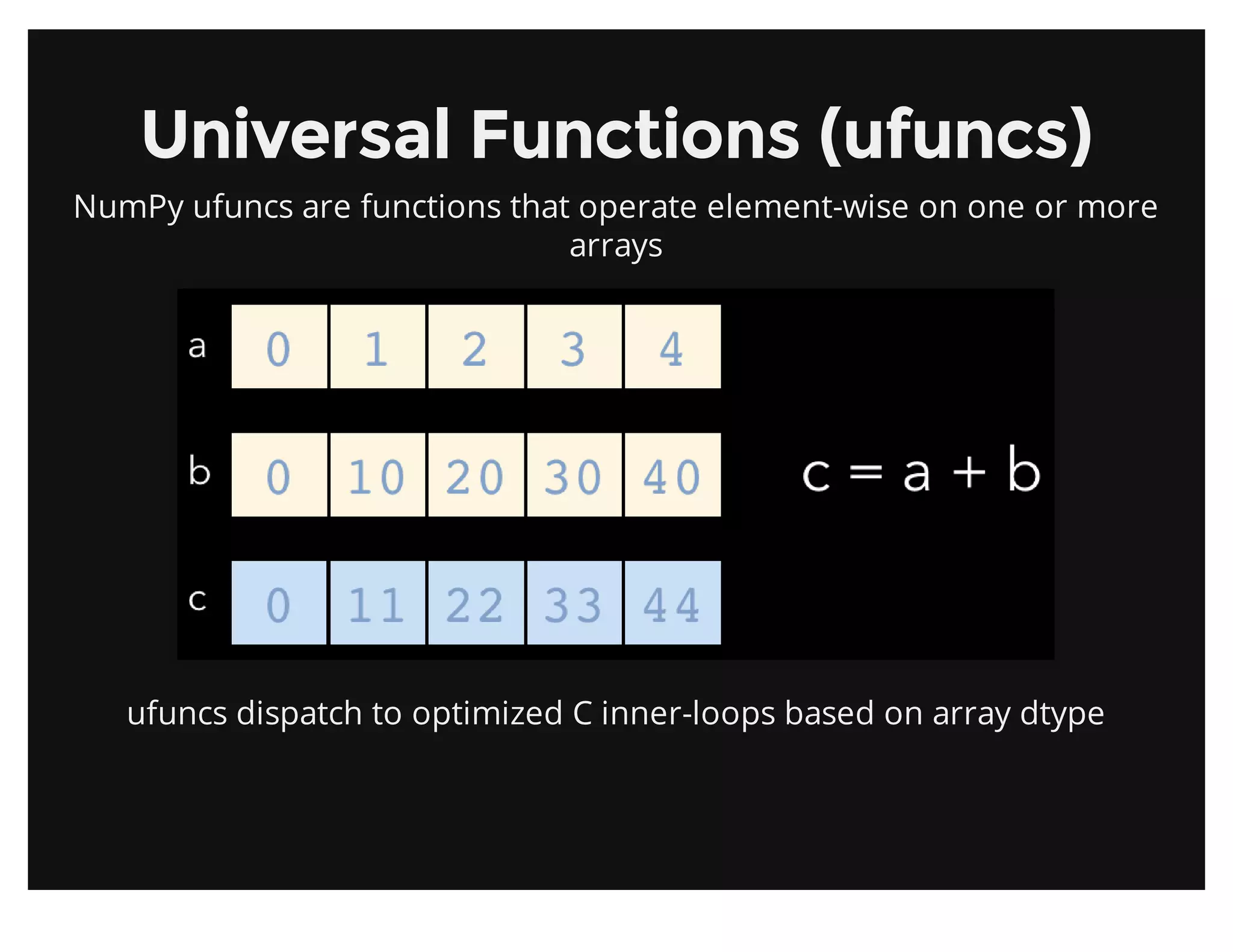
Here's a code example combining both:

import numpy as np




# Array of test failure counts from two different test suites
suite1_failures = np.array([5, 8, 2, 4])
suite2_failures = np.array([3, 10, 1, 5])




# Element-wise operation: Get total failures per test case
total_failures = suite1_failures + suite2_failures
print(f"Total failures per test case: {total_failures}")




# Scalar operation: Suppose each failure requires 0.5 hours to investigate
investigation_time = total_failures * 0.5
print(f"Investigation time in hours: {investigation_time}")

Output:

Total failures per test case: [ 8 18  3  9]
Investigation time in hours: [4.  9.  1.5 4.5]

Notice that we did not write any loops. NumPy handles the iteration efficiently in its underlying C code. Standard arithmetic operators like +, -, *, /, and ** (for exponentiation) all work this way.

A Quick Note on Multiplication: The * operator performs element-wise multiplication, not matrix multiplication. Matrix multiplication is a different operation used in linear algebra and is done using the @ operator or the np.dot() function. We'll touch on that if needed in later, more advanced lessons.

3. Broadcasting: Operations on Different-Sized Arrays

What happens if you try to perform an operation on two arrays of different shapes? Sometimes it fails, but often NumPy can still produce a result using a powerful mechanism called broadcasting.

Broadcasting describes how NumPy treats arrays with different shapes during arithmetic operations. Subject to certain constraints, the smaller array is "broadcast" across the larger array so that they have compatible shapes.

The rules for broadcasting are:

1. If the arrays do not have the same number of dimensions, prepend 1s to the shape of the smaller array until they do.
2. The size of each dimension must either be equal, or one of them must be 1.

If these conditions are met, the array with a dimension of size 1 is virtually "stretched" to match the size of the other array's corresponding dimension.

Practical Example: Normalizing Data

Imagine you have test scores for three candidates on four different skills. You want to subtract the average score for each candidate from their individual scores.

import numpy as np




# Scores for 3 candidates on 4 skills
scores = np.array([
    [80, 75, 90, 85],  # Candidate 1
    [95, 88, 80, 92],  # Candidate 2
    [70, 78, 85, 81]   # Candidate 3
])




# Calculate the average score for each candidate (average across rows)
avg_scores = np.mean(scores, axis=1)
print(f"Average scores per candidate: {avg_scores}")
print(f"Shape of scores: {scores.shape}") # (3, 4)
print(f"Shape of avg_scores: {avg_scores.shape}") # (3,) - a 1D array




# To broadcast, we need to make avg_scores a column vector (shape (3, 1))
# This makes it compatible for broadcasting with the (3, 4) scores array.
avg_scores_reshaped = avg_scores.reshape((3, 1))
print(f"Shape of reshaped avg_scores: {avg_scores_reshaped.shape}") # (3, 1)




# Broadcast the subtraction
normalized_scores = scores - avg_scores_reshaped
print("\nScores relative to each candidate's average:")
print(normalized_scores)

Output:

Average scores per candidate: [82.5 88.75 78.5 ]
Shape of scores: (3, 4)
Shape of avg_scores: (3,)
Shape of reshaped avg_scores: (3, 1)

Scores relative to each candidate's average:
[[ -2.5  -7.5   7.5   2.5]
 [  6.25  -0.75  -8.75   3.25]
 [ -8.5  -0.5   6.5   2.5]]

Here, the (3, 1) array of averages was broadcast across the (3, 4) array of scores. The average for the first candidate (82.5) was subtracted from all four of their scores, the average for the second (88.75) was subtracted from theirs, and so on.

4. Summarizing Data with Aggregation

Another common numerical task is to summarize data. For example, calculating the average response time of an API or finding the maximum memory used during a test run. NumPy provides fast functions for these "aggregation" operations.

Key aggregation functions include np.sum(), np.mean(), np.min(), np.max(), and np.std() (standard deviation).

A Testing Scenario

Let's analyze a set of API response times, recorded in milliseconds. We have data for 3 different endpoints, each tested 4 times.

import numpy as np




# Response times in ms for 3 endpoints over 4 test runs
# Rows = endpoints, Columns = test runs
response_times = np.array([
    [121, 125, 119, 123],  # Endpoint A
    [205, 250, 210, 208],  # Endpoint B
    [88, 92, 85, 90]       # Endpoint C
])




# Find the maximum response time recorded in the entire test session
max_overall_time = np.max(response_times)
print(f"Maximum overall response time: {max_overall_time} ms")




# Calculate the average response time for EACH endpoint
# We average across the columns (axis=1)
avg_time_per_endpoint = np.mean(response_times, axis=1)
print(f"Average response time per endpoint: {avg_time_per_endpoint.round(2)} ms")




# Calculate the average response time for EACH test run
# We average down the rows (axis=0)
avg_time_per_run = np.mean(response_times, axis=0)
print(f"Average response time per run: {avg_time_per_run.round(2)} ms")

Output:

Maximum overall response time: 250 ms
Average response time per endpoint: [122.  218.25  88.75] ms
Average response time per run: [138.   155.67 138.   140.33] ms

The axis parameter is very powerful. A helpful way to remember it is:

• axis=0: collapses the rows (aggregates "down" the columns).
• axis=1: collapses the columns (aggregates "across" the rows).

Conclusion

Great work! You've just taken a significant step into the world of high-performance computing in Python. NumPy is the bedrock of the data science and AI ecosystem, and the skills you've learned today will be used continuously as we move forward.

Key Takeaways

• NumPy Arrays (ndarray): A powerful data structure for fast, numerical computation, superior to Python lists for this purpose due to homogeneous types and contiguous memory.
• Vectorized Operations: NumPy allows you to perform operations like addition or multiplication on entire arrays at once without writing Python for loops.
• Scalar & Element-wise Arithmetic: You can perform operations between an array and a single number (array * 5) or between two arrays of the same shape (array1 + array2).
• Broadcasting: NumPy's mechanism for performing operations on arrays of different (but compatible) shapes by virtually "stretching" the smaller array.
• Aggregation: Functions like np.mean(), np.max(), and np.sum() allow for efficient summarization of data, with the axis parameter providing control over whether you aggregate along rows or columns.

What's Next?

While NumPy is fantastic for raw numerical data, it doesn't have a user-friendly way to handle labeled, tabular data—like what you'd find in a CSV file with headers. In our next lesson, we will introduce pandas, the premier library for data analysis in Python. You will learn to read, filter, and select data from pandas DataFrames, which will feel like working with powerful, programmable spreadsheets. You'll also see how pandas is built directly on top of the NumPy arrays you learned about today.