Mean-Field Decoupling and Self-Consistency

In our last lesson, we established the concept of the order parameter as a crucial tool for simplifying the description of a complex many-body system undergoing a phase transition. We learned how to identify a suitable order parameter by analyzing the symmetries broken during the transition. Now, we move from description to prediction. How can we build a theoretical model to calculate the behavior of this order parameter—for instance, how magnetization appears as a ferromagnet is cooled?

This lesson introduces mean-field theory (MFT), the foundational approximation method in the physicist's toolkit for tackling interacting many-body problems. The core idea is brilliantly simple yet powerful: instead of tracking the complex, fluctuating interactions each particle experiences from all its neighbors, we replace them with an average or "mean" field. This masterstroke transforms an intractable many-body problem into a collection of solvable single-body problems. You will learn how to perform this approximation, known as a mean-field decoupling, and derive the famous self-consistency equation that lies at the heart of the theory.

The Core Idea: Taming the Interactions

Let's consider a generic Hamiltonian for interacting spins, like the Ising model:

H = - \frac{1}{2} i, j \sum J_{ij} S_{i} S_{j} - i \sum h_{i} S_{i}

The term $S_{i} S_{j}$ couples the degrees of freedom on different sites, making this a genuine many-body problem. A direct solution would require summing over all $2^{N}$ configurations, which is impossible for a macroscopic system.

Mean-field theory's central move is to approximate this two-body interaction term. We decompose each spin operator $S_{i}$ into its statistical average (the local magnetization $m_{i} = ⟨ S_{i} ⟩$ ) and the fluctuation around that average, $δ S_{i} = S_{i} - m_{i}$ . The interaction term then becomes:

S_{i} S_{j} = (m_{i} + δ S_{i}) (m_{j} + δ S_{j}) = m_{i} m_{j} + m_{i} δ S_{j} + m_{j} δ S_{i} + δ S_{i} δ S_{j}

The mean-field approximation consists of assuming that the fluctuations are small and uncorrelated, allowing us to neglect the term that is quadratic in the fluctuations, $δ S_{i} δ S_{j}$ . This is the crucial decoupling step. The interaction is thus linearized:

S_{i} S_{j} \approx m_{i} m_{j} + m_{i} (S_{j} - m_{j}) + m_{j} (S_{i} - m_{i}) = m_{i} S_{j} + m_{j} S_{i} - m_{i} m_{j}

Let's see this approximation in action. The following video introduces the concept for the Heisenberg model and explains the physical intuition behind it.

Quantum phase transitions, spontaneous symmetry breaking, mean field theory

This video from Dr Mitchell's physics channel provides a clear, conceptual introduction to the mean-field approximation.

Watch the segment from 30:23 to 34:17. The key takeaway is how the original Hamiltonian, which is quadratic in the spin operators (representing interacting spins), is transformed into a mean-field Hamiltonian that is linear in the spin operators. This means each spin is now treated as being independent, interacting only with an effective magnetic field generated by the average behavior of its neighbors.

The Mean-Field Hamiltonian and the Self-Consistency Equation

By substituting our approximation $S_{i} S_{j} \approx m_{i} S_{j} + m_{j} S_{i} - m_{i} m_{j}$ into the original Hamiltonian, we obtain the mean-field Hamiltonian, $H_{M F}$ :

H_{M F} = - \frac{1}{2} i, j \sum J_{ij} (m_{i} S_{j} + m_{j} S_{i} - m_{i} m_{j}) - i \sum h_{i} S_{i}

After rearranging the terms (and using the symmetry $J_{ij} = J_{j i}$ ), this becomes:

H_{M F} = - i \sum S_{i} (h_{i} + j \sum J_{ij} m_{j}) + \frac{1}{2} i, j \sum J_{ij} m_{i} m_{j}

Look closely at this expression. It is a sum of single-spin terms, $H_{M F} = \sum_{i} H_{i}$ , plus a constant energy offset. Each spin $S_{i}$ now lives in an effective magnetic field:

h_{eff, i} = h_{i} + j \sum J_{ij} m_{j}

This effective field is the external field $h_{i}$ plus a contribution from all other spins, but this contribution depends only on their average magnetizations $m_{j}$ . The many-body problem has been decoupled into $N$ independent single-body problems, which we know how to solve from basic statistical mechanics.

This leads to a classic "chicken and egg" problem: to define the Hamiltonian, we need the average magnetizations ${m_{i}}$ . But to calculate the averages, we need the Hamiltonian. The solution is to demand self-consistency.

We calculate the average magnetization $m_{i}$ using the mean-field Hamiltonian itself. For a spin-1/2 system in an effective field $h_{eff, i}$ , the result is:

m_{i} = ⟨ S_{i} ⟩_{M F} = tanh (β h_{eff, i})

where $β = 1/ k_{B} T$ . Substituting the definition of $h_{eff, i}$ , we arrive at the self-consistency equations:

m_{i} = tanh (β (h_{i} + j \sum J_{ij} m_{j}))

This is a system of $N$ coupled non-linear equations for the local magnetizations ${m_{i}}$ . Solving them gives us the state of the system within mean-field theory.

To gain more solid footing with this derivation, let's turn to a set of lecture notes that walks through these same steps for the Ising model.

Statistical Physics (PHY831): Part 3 - Interacting systems

These notes from a Michigan State University statistical physics course offer a concise and formal derivation of the mean-field framework for the Ising model.

First, read Section A, "General spin half mean field theory" on page 2. This formalizes the fluctuation expansion and the decoupling approximation that leads to the mean-field Hamiltonian. Next, read Section B, "Mean field theory for spin half ferromagnet" on page 3. This specializes the general equations to a simple ferromagnet, where translational symmetry allows us to assume m_i = m for all sites, reducing the system of N equations to a single self-consistency equation for the global magnetization m, given as Eq. (15).

Solving the Self-Consistency Equation

For a simple ferromagnet with nearest-neighbor coupling $J$ on a lattice with coordination number $z$ , and in zero external field ( $h = 0$ ), the self-consistency equation simplifies to a single transcendental equation for the order parameter $m$ :

m = tanh (β z J m)

While we cannot write down a closed-form solution for $m$ , we can find the solutions graphically. We plot two functions of $m$ : $y = m$ and $y = tanh (\frac{z J}{k _{B} T} m)$ , and look for their intersection points.

High Temperature (T > T_c): When $T$ is large, the initial slope of the $tanh$ function, which is $z J / k_{B} T$ , is less than 1. The only intersection point is at $m = 0$ . This describes the paramagnetic phase, with no spontaneous magnetization.
Low Temperature (T < T_c): When $T$ is small, the initial slope $z J / k_{B} T$ is greater than 1. In this case, three intersection points appear: an unstable solution at $m = 0$ and two stable, symmetric solutions at $m = \pm m_{0}$ . The system spontaneously breaks the $m \to - m$ symmetry and settles into one of these states with non-zero magnetization. This is the ferromagnetic phase.
Critical Temperature (T = T_c): The transition occurs precisely when the slope at the origin changes from being less than 1 to greater than 1. The critical point is therefore found when the slope is exactly 1: $\frac{z J}{k _{B} T _{c}} = 1 ⟹ k_{B} T_{c} = z J$

The following resource provides a clear graphical illustration of this central result.

[PDF] Statistical Mechanics Lecture Set 7: Magnetism and its mean-field ...

These notes from the University of Colorado provide a concise overview of Weiss mean-field theory, which is historically synonymous with MFT for magnetism.

Focus on Fig. 4 and the associated discussion on pages 13-14. This visual analysis is fundamental to understanding how a non-zero order parameter solution emerges spontaneously as the system is cooled below its critical temperature.

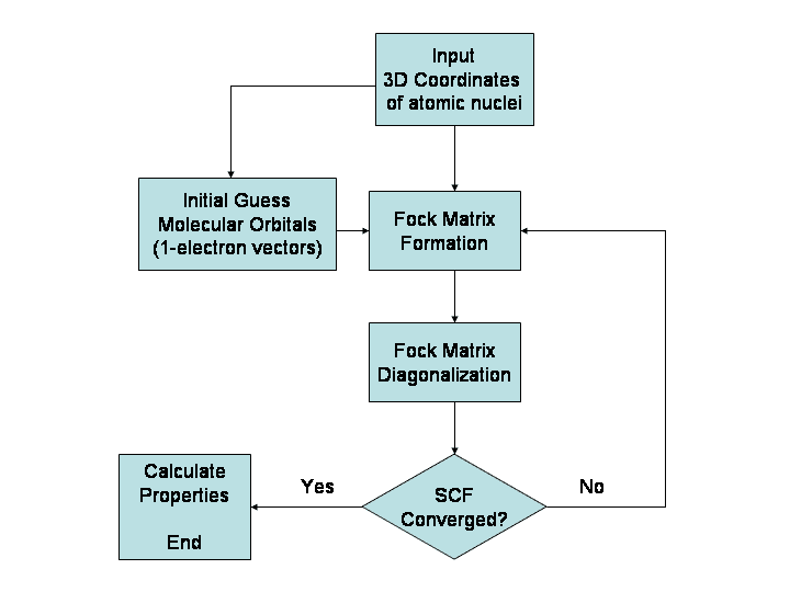
The process of starting with a guess for the order parameter, calculating a new value, and iterating until the input and output values match is the essence of a self-consistent field (SCF) calculation, a cornerstone of computational physics and chemistry.

A general flowchart for a self-consistent field calculation, widely used in computational chemistry and condensed matter physics. The core logic involves making an initial guess for some quantities (like molecular orbitals or, in our case, the mean field $m$), using them to construct an effective Hamiltonian (Fock Matrix), solving it, and then checking if the resulting output is consistent with the initial guess. If not, the process is iterated until convergence is reached. This is precisely the procedure for solving the mean-field self-consistency equation.

A Broader View: The Universality of the Method

The decoupling procedure you've learned is not limited to classical spin models. It is a general research methodology applicable across many domains of physics. Given your background in quantum field theory and condensed matter, you'll recognize its structure in the Hartree-Fock approximation, which is nothing more than a mean-field theory for interacting quantum particles like electrons.

In a system of interacting fermions, the interaction part of the Hamiltonian involves a product of four creation/annihilation operators, such as $c_{i}^{†} c_{j}^{†} c_{k} c_{l}$ . A mean-field decoupling, analogous to what we did for spins, approximates this four-operator term as a sum of two-operator terms multiplied by expectation values (the "mean fields").

The following video provides an advanced but conceptually clear derivation.

6- Mean-field theory - Course on Quantum Many-Body Physics

This segment from a course on Quantum Many-Body Physics extends the mean-field concept to interacting identical quantum particles. This provides a direct link between the simple Ising model MFT and the more sophisticated Hartree-Fock methods used in quantum chemistry and solid-state physics.

Watch the section from 34:01 to 1:09:16. The derivation is detailed, so focus on the overarching strategy rather than each algebraic step. The lecturer starts with a four-fermion interaction term and applies a decoupling scheme (akin to Wick's theorem for non-interacting states) to break it down. By writing operators as their average plus a fluctuation and neglecting the quadratic fluctuation terms, he derives an effective single-particle Hamiltonian. Notice the emergence of the "direct" (Hartree) and "exchange" (Fock) terms. This powerfully demonstrates that the same decoupling logic underpins both the simple spin model and the quantum electron gas.

This same methodology is also the basis for the van der Waals equation of state for real gases and the celebrated BCS theory of superconductivity, where the interaction between Cooper pairs is replaced by a mean field.

This image conceptually shows the progression from a fluctuating microscopic system to a smooth, macroscopic description. The first step, SCMF (Self-Consistent Mean Field), replaces the noisy, detailed interactions with a smooth average field, capturing the essence of the ordered state. This is precisely the approximation we have studied today. Subsequent theories, like Self-Consistent Field Theory (SCFT), build upon this to incorporate more sophisticated fluctuation effects.

Conclusion

In this lesson, we have moved from describing an ordered phase to calculating its properties. We have unlocked the core methodology of mean-field theory, one of the most versatile tools in the theoretical physicist's arsenal.

Key Takeaways:

Mean-field theory reduces a many-body problem to a single-body problem by replacing pairwise interactions with an interaction between a single particle and an effective average field produced by all other particles.
The key mathematical step is the decoupling approximation: $A B \approx ⟨ A ⟩ B + A ⟨ B ⟩ - ⟨ A ⟩ ⟨ B ⟩$ , which linearizes the Hamiltonian by neglecting quadratic fluctuation terms.
This procedure leads to a self-consistency equation, a non-linear equation for the order parameter (e.g., $m = tanh (β z J m)$ ) whose solution determines the macroscopic state of the system.
Solving the self-consistency equation (e.g., graphically) allows us to predict the existence of a phase transition and calculate the critical temperature, $T_{c}$ .
This methodology is general, forming the basis for approximations like Hartree-Fock theory in quantum mechanics.

We have successfully constructed a theory from a microscopic Hamiltonian. However, mean-field theory has its limitations, most notably its neglect of spatial correlations in fluctuations. This approximation becomes poor near the critical point, especially in low-dimensional systems. This begs the question: can we develop a theory for phase transitions that is independent of the microscopic details and perhaps more robust near $T_{c}$ ?

In our next lesson, we will explore Landau theory, a beautiful and powerful phenomenological approach that does just that. Instead of starting from a microscopic Hamiltonian, Landau theory constructs a model for the free energy as a function of the order parameter, based solely on general principles of symmetry and analyticity. This will provide a complementary and profound perspective on the physics of phase transitions.

Recommended resources

The Core Idea: Taming the Interactions

The Mean-Field Hamiltonian and the Self-Consistency Equation

Solving the Self-Consistency Equation

A Broader View: The Universality of the Method

Conclusion