Symmetry in Integrals and Matrix Elements

1. The Vanishing Integral Principle

The most fundamental way symmetry aids calculation is by telling us when an integral is zero without having to compute it. You are already familiar with the simplest version of this from introductory calculus: the integral of an odd function over a symmetric interval is always zero.

This concept generalizes beautifully with the tools of group theory. The core idea is that for an integral over all space to be non-zero, the integrand itself must be "totally symmetric" with respect to the symmetries of the system. In the language of group theory, the integrand must transform according to the totally symmetric irreducible representation of the group.

Consider a generic quantum mechanical matrix element, which is an integral of the form:

This integral represents the amplitude for a transition from an initial state ${\psi }_i$ to a final state ${\psi }_f$ induced by an operator $\hat{O}$. The "vanishing integral theorem" gives us a powerful condition for when this integral must be zero.

As the reading explains, the theorem states that the integral is non-zero only if the direct product of the irreducible representations ($\Gamma$) of its constituent parts contains the totally symmetric representation (${\Gamma }_{\text{sym}}$):

This rule is the foundation of all selection rules in quantum mechanics. It tells us which transitions are allowed by symmetry and which are strictly forbidden.

2. Selection Rules for Atomic Transitions

Let's apply this principle to a familiar problem: electric dipole transitions in a hydrogen-like atom. The atom possesses spherical symmetry (described by the group SO(3)) and inversion symmetry (parity). An initial state $|n,l,m⟩$ transitions to a final state $|n^{\prime },l^{\prime },m^{\prime }⟩$ via the dipole operator $\hat{\vec{d}}=-e\hat{\vec{r}}$. The matrix element is $⟨n^{\prime },l^{\prime },m^{\prime }|-e\hat{\vec{r}}|n,l,m⟩$.

Let's analyze this using two symmetries:

1. Parity: The atomic wavefunctions $|l,m⟩$ are eigenstates of the parity operator $\hat{\Pi }$ with eigenvalue $(-1{)}^l$. The operator $\hat{\vec{r}}$ is a vector, so it has odd parity (eigenvalue -1). For the integral to be non-zero, the integrand's total parity must be even:

   $$\begin{gathered} \Pi ({\psi }_{l^{\prime }{m}^{\prime }}^{\ast })\times \Pi (\hat{\vec{r}})\times \Pi ({\psi }_{lm})=(+1) \\ (-1{)}^{l^{\prime }}\times (-1)\times (-1{)}^l=(+1) \\ (-1{)}^{l^{\prime }-l+1}=(+1) \end{gathered}$$

   This implies that $l^{\prime }-l$ must be an odd integer. This gives us the parity selection rule: $\Delta l=\pm 1,\pm 3,\dots$. Transitions between states of the same parity (e.g., s $\to$ s, p $\to$ p, d $\to$ s) are forbidden.

2. Rotational Symmetry (SO(3)): The operator $\hat{\vec{r}}$ is a vector, which in the language of angular momentum is a rank-1 object. The states $|l,m⟩$ have angular momentum $l$. The transition involves combining the atom's initial angular momentum with the "angular momentum of the operator" to get the final angular momentum. The rules for adding angular momentum (the triangle inequality) require that:

   $$|l-1|\le l^{\prime }\le l+1$$

   Combining this with the parity rule ($\Delta l$ must be odd) gives the sharp selection rule for electric dipole transitions: $\Delta l=\pm 1$.

Furthermore, the components of the operator $\hat{\vec{r}}$ transform like specific spherical harmonics: $x\pm iy\sim Y_{1,\pm 1}$ and $z\sim Y_{1,0}$. If the transition is driven by light polarized along the z-axis, the operator is $\hat{z}$. The conservation of the z-component of angular momentum implies $m^{\prime }=m+0$, so $\Delta m=0$.

These ad-hoc arguments are powerful, but they are systematized and made far more general by the Wigner-Eckart theorem.

3. The Wigner-Eckart Theorem

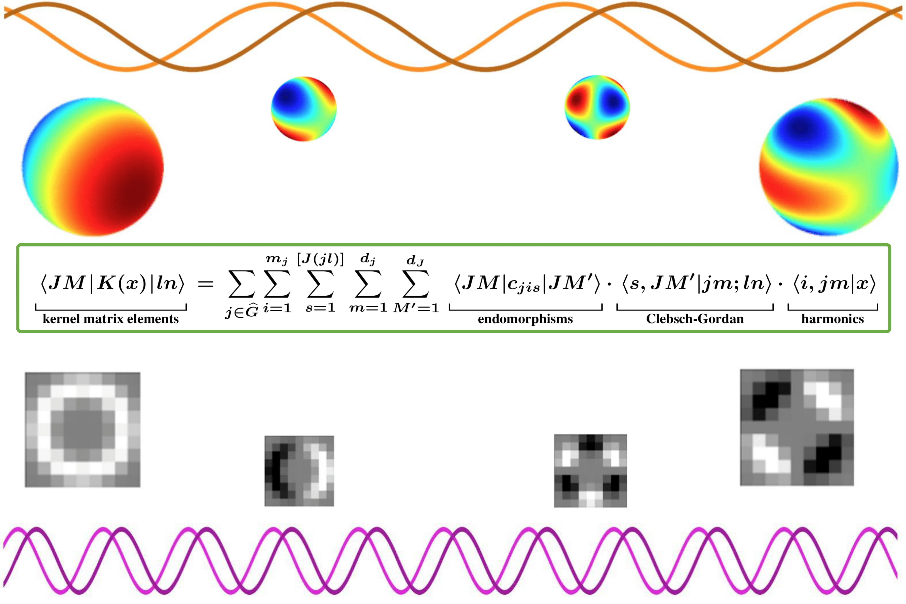
The Wigner-Eckart theorem is one of the most practical results of symmetry in quantum mechanics. It formalizes the "addition of angular momentum" picture we just used. It states that the matrix element of a spherical tensor operator can be factored into two parts:

1. A geometrical factor, called a Clebsch-Gordan coefficient, which depends only on the angular momentum quantum numbers ($j,m$) and is independent of the specific operator or the physics of the system. This factor contains all the selection rules.
2. A physical factor, called the reduced matrix element, which contains all the complex dynamics but is independent of the magnetic quantum numbers ($m,m^{\prime },q$).

Before stating the theorem, we need to understand its key ingredient.

With the concept of a spherical tensor operator $T_q^{(k)}$ in hand, we can appreciate the power of the Wigner-Eckart theorem.

Let's now turn to a more formal statement.

The theorem, as stated in the notes (Eq. 6.26), is:

Here, $C_{M{m}_1{m}_2}^{J{j}_1{j}_2}$ is the Clebsch-Gordan coefficient, and $⟨J||T^{(j_1)}||j_2⟩$ is the reduced matrix element.

The power of this theorem is immense. Suppose you need to calculate the $(2j_2+1)(2j_1+1)(2J+1)$ matrix elements for all possible magnetic quantum numbers. The theorem tells you they are all proportional. You only need to calculate one of them (for a convenient choice of m-values) and look up the Clebsch-Gordan coefficients in a table to find all the others.

4. Application: The Landé g-factor

A classic application that showcases the utility of the Wigner-Eckart theorem is the calculation of the Landé g-factor, which describes the energy splitting of atomic levels in a weak magnetic field (the Zeeman effect). Given your background in condensed matter, this should be a familiar context.

The perturbation to the Hamiltonian is $H^{\prime }={\mu }_B(\vec{L}+2\vec{S})\cdot \vec{B}$. The states of the atom are eigenstates of total angular momentum $|n,l,j,m⟩$. The challenge is to calculate the energy shift $E^{\prime }=⟨n,l,j,m|H^{\prime }|n,l,j,m⟩$. The difficult part is the matrix element of $\vec{S}$, since the states are not eigenstates of $S_z$.

This is where a corollary of the Wigner-Eckart theorem, often called the projection theorem, comes to the rescue. It states that within a manifold of states with a given total angular momentum $j$, the matrix elements of any vector operator $\vec{V}$ are proportional to the matrix elements of the total angular momentum operator $\vec{J}$ itself.

The proportionality constant $C$ is independent of the magnetic quantum numbers $m,m^{\prime }$. The proof of this is a direct application of the Wigner-Eckart theorem, as both $\vec{V}$ and $\vec{J}$ are rank-1 tensor operators.

This allows us to replace the tricky operator $\vec{S}$ with a proportional operator $\vec{J}$, whose matrix elements are simple.

This application is a perfect example of the research methodology you are aiming to master. A seemingly intractable calculation is rendered simple by identifying the correct symmetry principle and applying a powerful theorem, reducing the problem to algebraic manipulation of quantum numbers.

Conclusion

In this lesson, we have seen how symmetry is not just an abstract property of physical laws, but a practical and powerful tool for simplifying calculations.

Key Takeaways:

• The Vanishing Integral Theorem: A matrix element $⟨{\Psi }_f|\hat{O}|{\Psi }_i⟩$ can be non-zero only if the representation of the product of its components, $\Gamma ({\Psi }_f^{\ast })\otimes \Gamma (\hat{O})\otimes \Gamma ({\Psi }_i)$, contains the totally symmetric representation. This is the master principle behind all selection rules.
• Selection Rules: Symmetries like parity and rotation impose strict rules ($\Delta l=\pm 1$, $\Delta m=0,\pm 1$) that determine which transitions are allowed or forbidden.
• Wigner-Eckart Theorem: This theorem separates the "geometry" (Clebsch-Gordan coefficients) from the "dynamics" (reduced matrix elements) in a matrix element calculation. It allows us to determine all matrix elements for different magnetic quantum numbers by calculating just one, drastically reducing the workload.
• The Projection Theorem: A direct consequence of the Wigner-Eckart theorem, it allows us to replace any vector operator with the total angular momentum operator up to a constant of proportionality, greatly simplifying calculations within a $j$-multiplet.

You have now completed the module on Symmetry and Conservation Laws. You have seen how to identify symmetries, derive conservation laws via Noether's theorem, understand the consequences of symmetry breaking through Goldstone's theorem, and finally, how to use symmetry as a practical calculational tool.

In our next lesson, we will begin a new module on Constructing and Validating Toy Models. You will learn how to apply the principles we've discussed—symmetry, dimensional analysis, and physical intuition—to build simplified models that capture the essential physics of a complex phenomenon. The ability to derive selection rules will be crucial, as it tells you which interaction terms are forbidden by symmetry and can be excluded from your model from the outset.