Goldstone Modes: From Broken Symmetry to Observable Properties

1. Goldstone's Theorem: From Intuition to Statement

Let's begin by formalizing our intuitive picture. When a continuous symmetry is spontaneously broken, the system chooses a ground state from a continuous family of equivalent, degenerate states. These states form a manifold, often called the vacuum manifold.

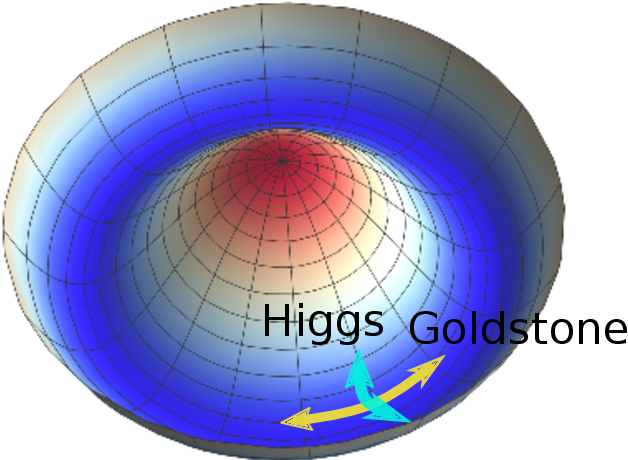
This leads to the central statement of Goldstone's theorem:

For every continuous global symmetry generator that is spontaneously broken, there appears a massless, spin-zero particle in the spectrum, known as a Nambu-Goldstone boson (or Nambu-Goldstone mode).

The core idea is that a long-wavelength fluctuation that slowly varies the order parameter along the vacuum manifold costs vanishingly small energy. This zero-energy excitation is the Goldstone mode.

2. Derivation for a U(1) Symmetry

To see this in action, let's return to the complex scalar field with a U(1) symmetry from our last lesson. The Lagrangian is:

The vacuum manifold is the circle of states where $|\varphi {|}^2={\mu }^2/\lambda =v^2$. We arbitrarily choose the vacuum to be the real, positive value $⟨\varphi ⟩=v$.

In the previous lesson, we analyzed the discrete $Z_2$ case by expanding the field as $\varphi (x)=v+\eta (x)$. For the continuous U(1) case, a more insightful approach is to parameterize the field in terms of its amplitude and phase. This is a key methodological step: choosing coordinates that respect the geometry of the problem simplifies the physics.

Let's represent the complex field $\varphi$ using two real fields: a radial field $R(x)$ for fluctuations in amplitude, and an angular field $\theta (x)$ for fluctuations in phase.

The ground state corresponds to $R(x)=\sqrt{2}v$ and $\theta (x)=\text{constant}$. We now expand around this vacuum by defining fluctuation fields $\eta (x)$ and $\zeta (x)$:

We will now substitute this into the Lagrangian and see what physics emerges for the $\eta$ and $\zeta$ fields.

As the derivation shows, after expanding around the vacuum, the Lagrangian for the fluctuation fields contains:

1. A Massive Radial Mode: The field $\eta (x)$, which represents fluctuations "up the walls" of the potential, acquires a mass $m_{\eta }^2=2{\mu }^2$. This is analogous to the massive particle we found in the discrete $Z_2$ case. In the context of the Standard Model, this would be the Higgs boson.
2. A Massless Angular Mode: The field $\zeta (x)$, which represents fluctuations "along the trough" of the potential, appears in the Lagrangian only with derivatives. There is no ${\zeta }^2$ term. The Lagrangian for $\zeta$ is of the form $\frac{1}{2}({\partial }_{\mu }\zeta {)}^2+\dots$, which describes a massless particle. This is the Nambu-Goldstone boson.

The U(1) symmetry isn't gone; it's hidden. It now manifests as an invariance of the Lagrangian under a constant shift $\zeta (x)\to \zeta (x)+\text{const}$. A potential term like $\frac{1}{2}{m}^2{\zeta }^2$ would violate this shift symmetry, which is why the Goldstone boson must be massless.

3. Properties of Goldstone Modes: Counting and Dispersion

Goldstone's theorem is more powerful than just predicting existence. A more refined analysis allows us to predict the number of NG modes and their dispersion relation (the relationship between energy $E$ and momentum $k$). This is particularly important in non-relativistic systems like those you study in condensed matter physics.

The key insight is that while the number of broken symmetry generators, $n_{BG}$, sets the upper bound for the number of NG modes, the actual number, $n_{NG}$, can be smaller. The general counting rule is:

Let's break this down:

• $n_{BG}$ is the number of broken generators. For a symmetry group $G$ broken to a subgroup $H$, this is simply $\text{dim}(G)-\text{dim}(H)$.
• ${\rho }_{ab}$ is a matrix defined by the expectation value of the commutator of the broken charge densities in the ground state: $${\rho }_{ab}\equiv -i⟨0|[Q_a,q_b(0)]|0⟩=\sum _c{f}_{ab}^c⟨q_c(0)⟩$$ where $Q_a$ are the conserved charge operators, $q_b(0)$ are the charge densities at the origin, and $f_{ab}^c$ are the structure constants of the Lie algebra. The crucial physical point is that ${\rho }_{ab}$ is non-zero only if the ground state has a non-zero density for some conserved charge.

This leads to a classification of NG modes into two types.

As the reading explains, the classification is as follows:

• Type A NG modes: These arise from broken generators that are not "paired up" by the $\rho$ matrix. The number of type A modes is $n_A=n_{BG}-\text{rank}(\rho )$. They typically have a linear dispersion relation, $E\propto |k|$, in the low-energy limit. In relativistic theories, ${\rho }_{ab}$ is always zero, so all NG modes are Type A, and $n_{NG}=n_{BG}$.

• Type B NG modes: These arise when pairs of broken generators become canonically conjugate due to a non-zero ${\rho }_{ab}$. The number of type B modes is $n_B=\frac{1}{2}\text{rank}(\rho )$. Each pair of broken generators produces a single NG mode. They typically have a quadratic dispersion relation, $E\propto |k{|}^2$.

This distinction is precisely what allows us to understand the different behaviors of low-energy excitations in various physical systems.

4. Application: Magnons in a Ferromagnet

Let's apply this powerful methodology to a canonical example from your field of interest: a ferromagnet.

Consider a simple Heisenberg model, where the interactions are invariant under the SO(3) group of spin rotations.

• Symmetry: The Hamiltonian has SO(3) symmetry, generated by the total spin operators $S_x,S_y,S_z$.
• Ground State: At low temperatures, the system chooses a ground state where all spins align along a specific, arbitrary direction. Let's say this is the z-direction. The ground state has a non-zero magnetization $⟨\vec{S}⟩=(0,0,M)$.
• Symmetry Breaking: This ground state is invariant under rotations about the z-axis (generated by $S_z$) but not under rotations about the x or y axes. Therefore, the symmetry is spontaneously broken from $G=\text{SO(3)}$ to $H=\text{SO(2)}$.
• Broken Generators: The generators $S_x$ and $S_y$ are broken. So, $n_{BG}=\text{dim(SO(3))}-\text{dim(SO(2))}=3-1=2$.
• Calculate ${\rho }_{ab}$: We need to check the commutator of the broken generators in the ground state. The relevant structure constant is from $[S_x,S_y]=i{S}_z$. $${\rho }_{xy}\propto ⟨0|[S_x,S_y]|0⟩=i⟨0|S_z|0⟩\propto iM\ne 0$$ The matrix $\rho$ has off-diagonal entries, and its rank is 2.
• Count the NG modes: Using the formula: $$n_{NG}=n_{BG}-\frac{1}{2}\text{rank}(\rho )=2-\frac{1}{2}(2)=1$$
• Classify the Mode: Since $\text{rank}(\rho )=2$, we have $n_B=\frac{1}{2}(2)=1$ and $n_A=2-2=0$. The two broken generators, $S_x$ and $S_y$, pair up to produce a single Type B NG mode.

Prediction: The low-energy spectrum of a ferromagnet should contain one NG mode with a quadratic dispersion relation, $E\propto k^2$. This is precisely the magnon, or spin wave.

Conclusion

In this lesson, you have learned how to move from the general concept of spontaneous symmetry breaking to making concrete, testable predictions about a system's low-energy behavior.

Key Takeaways:

• Goldstone's Theorem guarantees that the spontaneous breaking of a continuous global symmetry results in massless Nambu-Goldstone (NG) modes.
• The properties of these modes are determined by the symmetry breaking pattern $G\to H$ and the properties of the ground state.
• The number of NG modes is given by the general counting rule $n_{NG}=n_{BG}-\frac{1}{2}\text{rank}({\rho }_{ab})$, where ${\rho }_{ab}$ depends on the ground state's charge density.
• NG modes are classified into Type A (typically linear dispersion, $E\propto |k|$) and Type B (typically quadratic dispersion, $E\propto |k{|}^2$).
• This framework provides a powerful, systematic methodology to predict the existence and properties of low-energy excitations in diverse physical systems, from superfluids and magnets to the fundamental particles of nature.

In our next lesson, we will explore another practical application of symmetry principles. Having seen how symmetries (and their breaking) dictate the very particle content of our theories, we will now learn how to leverage those same symmetries to simplify complex calculations, such as evaluating integrals and matrix elements.