Welcome back. Last time, you counted seats by finding the winner in each single-member district, rather than awarding seats according to the overall vote total. You also saw that a party can win close races in several districts while its opponent wins fewer districts by large margins.
This lesson keeps voters and their preferences in the same places. Only the district boundaries change. You will see how packing concentrates an opposing party’s voters into a small number of districts, leaving that party with fewer seats than it won under another map. Allow about 35–40 minutes, including time to trace the maps and check the district totals.
What packing changes—and what it does not
Imagine that you draw districts for the Orange party. A Blue supporter remains a Blue supporter wherever you put the boundary; drawing a line does not create, remove, or move a vote. What you can change is which voters share a district.
Packing places many opposing voters together in districts they win by large margins. Those voters still elect representatives. But a district awards only one seat, whether the winner receives a narrow majority or nearly every vote. Concentrating Blue voters in one district can therefore leave fewer Blue voters available to form majorities in other districts.
Watch the packing portion of Gerrymandering: Is Geometry Silencing Your Vote? from Above The Noise for a quick visual version of that idea.
Gerrymandering: Is Geometry Silencing Your Vote?
Watch the whiteboard demonstration to see how a boundary can concentrate opposing voters while leaving nearby districts more favorable to the map drawer's party.
In the whiteboard segment, start at packing boundaries, just as the presenter turns from cracking to packing. Focus on the district the presenter is willing to lose heavily and on what that concentration does to the surrounding districts. We will check the mechanism with explicit voter counts below.
The Brennan Center for Justice’s Gerrymandering Explained supplies a concise definition. Read the technique descriptions for context, keeping the focus on packing for now.
Gerrymandering Explained | Brennan Center for Justice
Read the Brennan Center for Justice's account of how packing concentrates disfavored voters. Its adjacent description of cracking helps distinguish the two techniques, though cracking is the subject of the next lesson.
Under “There are multiple ways to gerrymander,” begin with the paragraph starting “The easiest way to understand gerrymandering” and read through the paragraph ending “both may be deployed by map drawers to engineer a decided partisan advantage.” In particular, follow the packing explanation: the packed group wins where it is concentrated, but has less voting strength in other districts.
The definition tells us what to look for. A small map lets us verify that it actually happens without assuming that a statewide vote share determines the seats.
A fixed electorate, drawn two ways
Consider a five-by-five grid containing 25 voters. Each square holds one voter, and every voter casts a ballot for either Blue or Orange. The three left columns contain Blue voters; the two right columns contain Orange voters. Thus Blue has 15 voters, or 60%, and Orange has 10, or 40%.
The map must have five districts of five voters each. Every district elects one representative by plurality. In the tables, the letter is the voter’s unchanging party preference; the number is the district to which that voter is assigned.
First, draw five vertical districts—one column per district:
| Row | Column 1 | Column 2 | Column 3 | Column 4 | Column 5 |
|---|---|---|---|---|---|
| 1 | B1 | B2 | B3 | O4 | O5 |
| 2 | B1 | B2 | B3 | O4 | O5 |
| 3 | B1 | B2 | B3 | O4 | O5 |
| 4 | B1 | B2 | B3 | O4 | O5 |
| 5 | B1 | B2 | B3 | O4 | O5 |
Districts 1, 2, and 3 each contain five Blue voters, so Blue wins three seats. Districts 4 and 5 each contain five Orange voters, so Orange wins two seats.
Now keep every letter in exactly the same square, but redraw the district boundaries. The new numbers show the new districts:
| Row | Column 1 | Column 2 | Column 3 | Column 4 | Column 5 |
|---|---|---|---|---|---|
| 1 | B1 | B2 | B3 | O3 | O3 |
| 2 | B1 | B2 | B3 | O3 | O4 |
| 3 | B1 | B2 | B4 | O4 | O4 |
| 4 | B1 | B2 | B4 | O5 | O5 |
| 5 | B1 | B2 | B5 | O5 | O5 |
Trace each number across adjacent squares. Every district remains one connected piece with exactly five voters. Districts 1 and 2 each hold five Blue voters: Orange has drawn two districts that Blue wins overwhelmingly. The other three districts contain smaller groups of Blue voters alongside Orange majorities.
| New district | Blue voters | Orange voters | Seat won by |
|---|---|---|---|
| 1 | 5 | 0 | Blue |
| 2 | 5 | 0 | Blue |
| 3 | 2 | 3 | Orange |
| 4 | 2 | 3 | Orange |
| 5 | 1 | 4 | Orange |
| Total | 15 | 10 | Blue: 2; Orange: 3 |
The totals are an important check: the electorate is still 15 Blue and 10 Orange. The district populations are still equal. Yet Blue’s seat count has fallen from three to two, while Orange’s has risen from two to three.
What did Orange gain by placing ten Blue voters in Districts 1 and 2? Blue wins those seats, but its margins of five votes to zero cannot earn additional seats. Across Districts 3–5, the remaining five Blue voters do not form a majority anywhere. This is packing’s distinctive trade-off: concede a few districts by large margins to improve your prospects in more districts elsewhere. The example shows what such a boundary arrangement can accomplish; it does not imply that every unequal seat outcome was deliberately engineered.
Recognizing the same mechanism on a larger map
The figure below holds 50 residents fixed: 30 Blue and 20 Orange. It divides them into five equal-population districts of ten residents each. Compare Map 1, with vertical districts, to Map 3. Keep your attention on the unchanged colored squares as you trace the changed black boundaries.
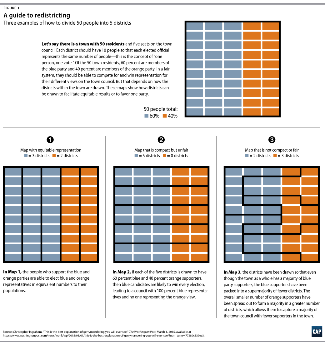
In Map 1, each party wins a number of districts matching its share of the town’s residents. In Map 3, Blue remains the larger group town-wide but wins only two of five seats. As in the worked grid, the relevant observation is where Blue voters end up concentrated, not a change in how many Blue voters exist.
The figure also illustrates a useful caution about appearances. A map’s shape alone does not tell you which party wins each district. Read the voters inside the boundaries, check that districts are equally populated, and count the winners. Later lessons will examine other criteria for evaluating maps; the seat reversal here establishes the mechanism, not a complete fairness judgment.
Key takeaways
Packing concentrates an opposing party’s voters into a small number of districts. They can win those districts decisively, but extra votes beyond those needed to win do not produce extra seats. In the worked example, both maps contain the same 15 Blue and 10 Orange voters in the same locations, and every district has five voters. Changing only the boundaries changes the result from three Blue seats and two Orange seats to two Blue seats and three Orange seats.
Next, you will examine cracking. Rather than concentrating opposing voters into districts they win overwhelmingly, cracking divides them among districts where they cannot assemble enough votes to win.