Welcome to the beginning of your course on mastering large-scale distributed systems. Your extensive experience in software engineering provides a fantastic foundation, and our goal throughout this journey is to build upon that by exploring the specific challenges and patterns essential for designing, operating, and leading at the scale of a company like Databricks.
We'll begin with Module 7, "Observability," because understanding a system's internal state is a prerequisite for making it reliable and performant. In a complex distributed environment, you can't fix what you can't see. This lesson introduces a cornerstone of modern observability: distributed tracing. We will demystify how to follow a single request through a maze of microservices by explaining the core concepts of traces, spans, and the critical mechanism of context propagation. This will lay the groundwork for the hands-on instrumentation you'll perform in the next lesson.
From Stack Trace to Distributed Trace
In your career, you've likely spent countless hours debugging applications. With monolithic systems, a stack trace is often your most powerful tool. It gives you a clear, sequential history of function calls within a single process that led to an error.
But what happens in a microservices architecture? A single user action, like adding an item to a cart, might trigger a chain reaction involving an API gateway, an authentication service, a product catalog service, an inventory service, and a cart service. These are all separate processes, often running on different machines. A traditional stack trace is confined to a single service and is blind to the larger, cross-service workflow. Debugging becomes a forensic exercise of piecing together clues from disparate log files, trying to correlate timestamps and request IDs manually. This is slow, frustrating, and often inconclusive.
Distributed tracing was created to solve this very problem. It provides the "stack trace" for a distributed architecture.
The Anatomy of a Request: Traces and Spans
At its heart, distributed tracing reconstructs the entire journey of a request as it propagates through a system. This journey is called a trace. Each step or unit of work within that journey is called a span.
To build a mental model, let's start with a foundational article.
This article provides a clear, high-level introduction to the core ideas. As you read, focus on building a solid conceptual understanding of traces and spans.
First, read the introductory sections, from the beginning through the definition of a distributed trace. This will frame the problem and the solution. Next, jump to the "Core Concepts and Components" section and read the definitions for Traces and Spans. Pay close attention to the properties of a span (ID, parent ID, timestamps, etc.). Finally, read the FAQ entry that asks, "What is distributed tracing...". This provides a concise summary to solidify your understanding.
As the article explains, a trace is the entire end-to-end story of a request, identified by a globally unique trace ID. It's composed of one or more spans. A span represents a single, timed operation, like an HTTP request to a specific service or a database query. Each span contains its own unique span ID and crucially, a reference to its parent span ID, creating a causal hierarchy.
The following video offers a great visual explanation of this relationship.
Distributed Tracing Explained: Understanding Microservice Observability
This short video from The Coding Gopher, "Distributed Tracing Explained," illustrates how a request path translates into a visual timeline of spans.
Watch from the beginning until the end of the spans explanation. Notice how the tree-like call graph on the left is transformed into the Gantt chart-style timeline on the right.
The relationship between the request path and the resulting trace is shown in the diagram below. The request originates from the user and hits service A. Service A then calls services B and E. Service B, in turn, calls C and D. This creates a hierarchy.

The trace visualization on the right shows how this hierarchy unfolds over time. Span A is the parent span (or root span); it represents the entire lifetime of the initial request. Spans B, C, D, and E are child spans. Notice that B and E start after A, and C and D start after B. The length of each bar represents its duration. This visualization immediately helps identify which operations are sequential and which are parallel, and where time is being spent.
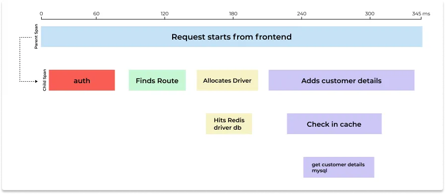
This timeline view is the primary tool you'll use to diagnose latency. If a request is slow, you can instantly see which span is the culprit. In the example above, the "Adds customer details" span, along with its sub-operations, takes up the majority of the request time.
The Secret Ingredient: Context Propagation
We've established that spans are linked together using parent-child relationships to form a trace. But how does this information travel between completely separate services? A call from Service A to Service B is just an HTTP request or a message on a queue. How does Service B know it's part of a trace started by Service A?
The answer is context propagation.
When Service A is about to call Service B, its tracing library captures the current tracing information—the trace ID and its own span ID—into an object called the context. It then injects, or propagates, this context into the outgoing request. When Service B receives the request, its tracing library extracts the context and uses it to create a new span. This new span in Service B will:
- Share the same
trace ID. - Set its
parent span IDto thespan IDit received fromService A.
This simple mechanism is the glue that stitches the distributed trace together. The OpenTelemetry documentation provides the standard definition for this concept.
This document from the official OpenTelemetry project formalizes the concepts of context and propagation.
Read the sections defining Context and Propagation. Then, review the Example to see how these concepts apply to a real-world scenario involving HTTP headers.
For network protocols like HTTP, context is most commonly propagated using request headers. The W3C Trace Context specification standardizes this with the traceparent header, ensuring that traces can be propagated across services even if they use different tracing libraries or vendors.
The following video provides a brilliant, practical demonstration of what happens when context propagation is missing and how adding it fixes the problem.
OpenTelemetry: How distributed tracing really works with Python, FastAPI and requests
This video, "OpenTelemetry: How distributed tracing really works," walks through a Python example to show the direct impact of context propagation.
Watch from the first run where the two services produce separate, disconnected traces in the Jaeger UI. This clearly shows the problem caused by a lack of context propagation. Next, watch the segment explaining the fix and the traceparent header. The author introduces a library that automatically adds the header. Pay close attention to the breakdown of the traceparent header format (version-trace_id-parent_id-trace_flags). This is the key mechanical detail. Finally, listen to the author's summary from stitching traces together where he defines "context" and "propagation mechanism" in his own words.
As the video demonstrates, without propagation, each service starts a new trace, resulting in fragmented, useless data. Once the traceparent header is added to the request from app one to app two, the tracing library in app two recognizes it, extracts the context, and correctly creates a child span. The result is a single, unified trace in the Jaeger UI.
Conclusion
In this lesson, you've learned the fundamental theory behind distributed tracing, a critical capability for operating modern, large-scale systems. Let's recap the key concepts:
- Distributed Tracing: A method to monitor requests as they flow across microservices, providing end-to-end visibility that is impossible with traditional logging and monitoring alone.
- Trace: Represents the entire journey of a single request through the system. It is defined by a unique
Trace ID. - Span: Represents a single, named, and timed unit of work within a trace (e.g., a call to one service). Spans are linked in a parent-child hierarchy to form the trace.
- Context Propagation: The mechanism that passes tracing information (the context, containing at least the
Trace IDandParent Span ID) between services. For HTTP, this is typically done via thetraceparentheader, as standardized by the W3C.
These concepts are the building blocks of observability in distributed architectures. Understanding them is the first step toward rapidly diagnosing latency, tracking down errors, and truly understanding your system's behavior.
In our next lesson, we will move from theory to practice. You will get hands-on experience instrumenting a sample microservice application using the OpenTelemetry SDK to generate your own trace data.