Analyzing Loop Time Complexity

From Operation Counting to Asymptotic Analysis

In our last session, we saw that precisely counting every single operation (e.g., $T(N)=27N+7$) is tedious and ultimately unnecessary for understanding an algorithm's scaling behavior. The power of asymptotic notation is that it allows us to ignore constant factors and lower-order terms, focusing only on the dominant term that dictates growth as the input size, $N$, becomes large.

This leads to a much more practical, simplified approach to analysis. We will develop a set of rules for analyzing common code structures. Let's begin with the most fundamental building block: the single loop.

Rule 1: Analyzing Single Loops

The most common pattern you'll encounter is a loop that iterates a number of times proportional to the input size.

A great way to transition from detailed counting to simplified analysis is presented in the lecture notes from Cornell University's CS 2110 course. Please read the following sections, which first perform a detailed operation count on two example methods and then introduce the simplified rules we'll be using.

As you saw, the general rules for single loops are:

• Linear Complexity $O(N)$: A loop is linear if its counter variable is incremented or decremented by a constant amount in each iteration (e.g., i++, i--, i += 5). The loop will run approximately $N/c$ times, which is $O(N)$. The paritySplit method is a perfect example.
• Constant Complexity $O(1)$: A loop has constant time complexity if it runs a fixed number of times, regardless of the input size N. For example, for (int i = 0; i < 100; i++).

Rule 2: Analyzing Nested Loops

When one loop is placed inside another, their complexities are multiplied.

The simplest case is when both the outer and inner loops run $N$ times. The inner loop's body will execute $N\times N=N^2$ times, resulting in $O(N^2)$ complexity.

A slightly more complex, but very common, pattern is when the inner loop's number of iterations depends on the outer loop's counter. Let's analyze the hasDuplicates method from the Cornell notes, which exemplifies this.

The video below, by Abdul Bari, provides a helpful visual walkthrough of this exact analysis, tracing the values of i and j and showing how the sum of the series builds up.

Rule 3: Analyzing Logarithmic Loops

Not all loops are linear. Consider a loop where the counter variable is multiplied or divided by a constant in each step.

// Example 1: Multiplication
for (int i = 1; i < n; i *= 2) {
    // constant time work
}

// Example 2: Division
for (int i = n; i > 0; i /= 2) {
    // constant time work
}

How many iterations do these loops perform?

• In Example 1, i takes values 1, 2, 4, 8, 16, ..., until it reaches n. This is asking, "How many times do we multiply 1 by 2 to get n?" The answer is ${\log }_{2}N$.
• In Example 2, i takes values n, n/2, n/4, ..., until it reaches 1. This is asking, "How many times do we divide n by 2 to get 1?" The answer is also ${\log }_{2}N$.

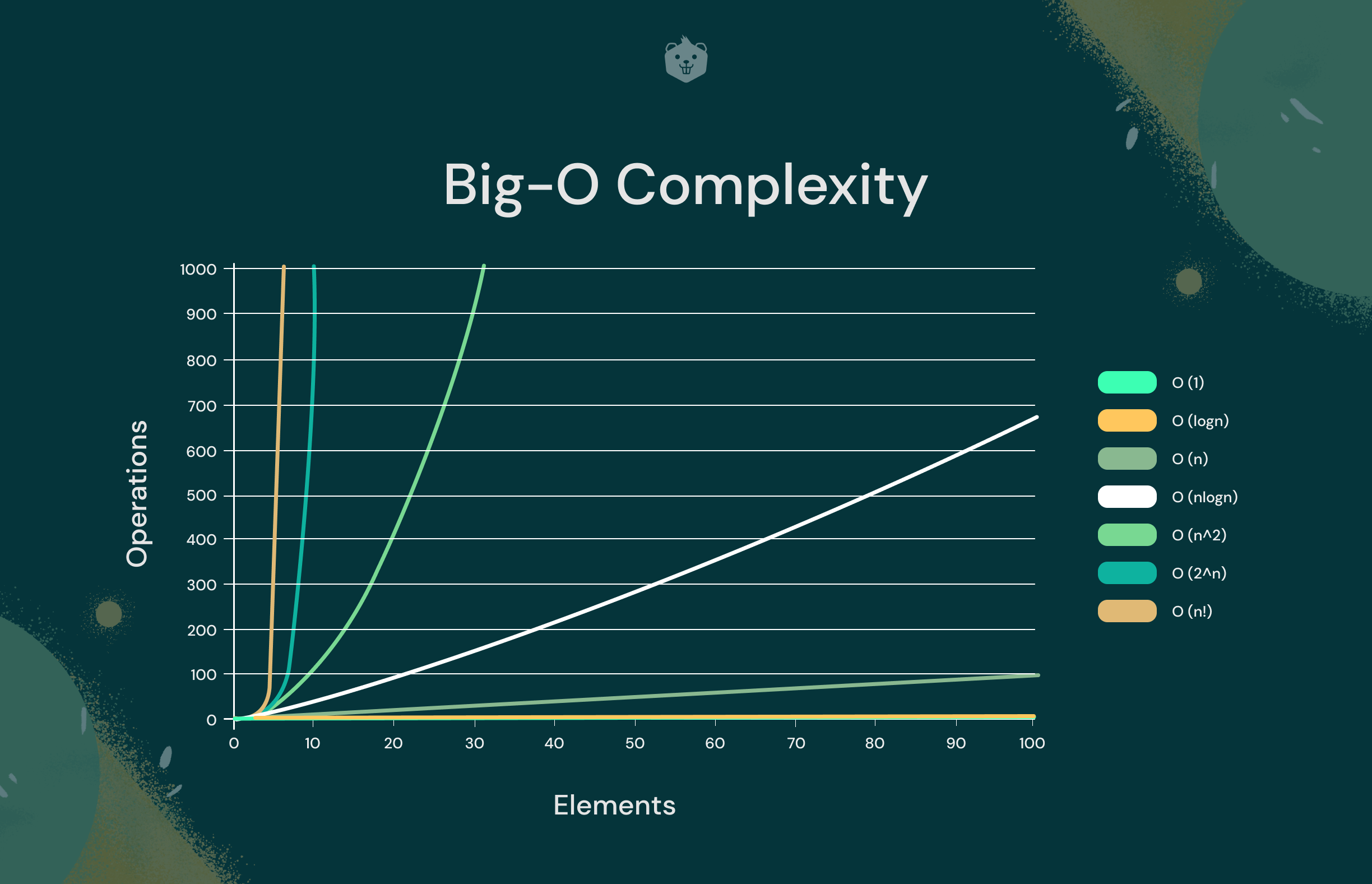
These loops have logarithmic time complexity, $O(\log N)$. This is a significant improvement over linear time. For an input of size 1 million, an $O(N)$ algorithm takes ~1 million steps, while an $O(\log N)$ algorithm takes only ~20 steps.

The following video provides an excellent and clear explanation of this concept.

Rules for Combinations

Now we can combine these basic rules:

• Sequential Loops: If you have loops that run one after another (sequentially), you add their complexities. The largest term dominates.
  • $O(N)+O(N)=O(2N)\to O(N)$
  • $O(N)+O(N^2)=O(N^2)$
• Nested Loops: If loops are nested, you multiply their complexities.
  • Outer loop $O(N)$, inner loop $O(\log N)$ $\to$ Total: $O(N\log N)$
  • Outer loop $O(N)$, inner loop $O(N)$ $\to$ Total: $O(N^2)$

Let's Practice

Your background in designing software flows will be useful here, as analyzing complexity is about understanding the flow of execution. Let's apply these rules to a few examples from the Cornell exercises.

Analysis of Practice Problems:

1. variance(int[] a):

   • This method contains a single for loop that runs from i = 0 to a.length - 1.
   • This is a classic linear loop. The work inside the loop (additions, multiplications, array access) is all $O(1)$.
   • The operations after the loop are also $O(1)$.
   • Complexity: $O(N)$, where $N$ is a.length.

2. bar(int[] a):

   • This method has three nested loops.
   • The outer loop runs $N$ times (i from 0 to $N-1$).
   • The second loop runs approximately $N$ times in the worst case (j from i to $N-1$).
   • The innermost loop runs a constant 100 times. This is an $O(1)$ loop.
   • Multiplying the complexities: $O(N)\times O(N)\times O(1)=O(N^2)$.
   • Complexity: $O(N^2)$.

3. numGreaterThan(int[] a, int[] b):

   • This is a fascinating case. It looks like a standard nested loop, which might lead you to guess $O(M\times N)$, where $M$ is a.length and $N$ is b.length.
   • However, look closely at the inner while loop's counter, j. It is not reset with each iteration of the outer for loop.
   • The for loop pointer i moves from 0 to M-1 (total of M steps).
   • The while loop pointer j moves from 0 to N-1 over the entire lifetime of the method call (total of N steps).
   • Since each pointer traverses its respective array only once, the total number of fundamental steps is proportional to the sum of the array lengths.
   • Complexity: $O(M+N)$. This is a common and efficient pattern, often called a "two-pointer" approach.

4. method3(int[] nums):

   • This method has a for loop that iterates $N$ times.
   • Inside the loop, it calls binarySearch. In the previous section of the Cornell notes, we saw that binarySearch has a complexity of $O(\log N)$ because it repeatedly halves the search space.
   • We have an $O(\log N)$ operation being performed $O(N)$ times.
   • Multiplying the complexities: $O(N)\times O(\log N)$.
   • Complexity: $O(N\log N)$.

Conclusion

In this lesson, we transitioned from the theory of asymptotic notation to the practical skill of analyzing iterative code. By establishing a few core rules, you can now quickly and effectively determine the time complexity of many common algorithms.

Here are the key takeaways:

• Single Linear Loops ($O(N)$): The loop counter changes by a constant amount.
• Nested Loops ($O(N^2)$): Complexity is found by multiplying the complexities of the outer and inner loops. Be wary of dependent loops and loops with non-resetting counters.
• Logarithmic Loops ($O(\log N)$): The loop counter changes by a multiplicative or divisive factor.
• Sequential Loops: Add complexities; the highest order term dominates.

You now have the tools to analyze how an algorithm scales. In our next lesson, we will focus on comparing these common complexity classes—O(1), O(log n), O(n), O(n log n), O(n²), and O(2^n). This will build your intuition for why choosing an O(N log N) algorithm over an O(N^2) one can be the difference between a program that is lightning-fast and one that is unusably slow.